
Data exhaust is increasing exponentially, and the variety and volume of this data has shown no indication of slowing down. Even the lowly Ubuntu OS or simple containerized workload running in Kubernetes can produce all sorts of user, system, infrastructure, authentication, and networking logs. This data increase necessitates security teams become SecDataOps teams.
By using a data lake to disaggregate storage from compute and adopting an open table format such as Apache Iceberg, you can set your SecDataOps teams up for success by scaling access to all relevant security and security-adjacent data. There is no doubt that Apache Iceberg will prove to be an asset in the weeks and months to come. It is a technology meant for these petabyte-scale workloads.
In this blog you will uncover (data engineering) challenges to building security data lakes and learn how to use Apache Iceberg to circumvent some of those challenges. You will explore the open table format, learn how to build Iceberg tables using Amazon Athena, and interact with them by inserting data, changing columns, changing values, performing time-travel queries, and more!
This blog is long, so here are a few shortcut links if you know what you’re looking for:
- Building a Data Lake and Its Challenges
- Partitions, Predicates, and File size
- Enter: Apache Iceberg
- Nine Benefits of Iceberg (on Amazon Athena)
- Building an Iceberg Table
- Generating and Migrating Data to Iceberg
- Working With Iceberg tables
So, What Is a Data Lake?
Data lakes have become just as ubiquitous of a term in security functions as zero trust and AI security. While the latter concepts have become ambiguous catch-alls, data lakes are well-defined and in common use.
In the simplest terms, a data lake is a central repository where data can be stored in its native (or normalized) format no matter if the data is unstructured, semi-structured, or structured. There is typically a metadata management service alongside the lake to enable cataloging of data types, serialization, and partitioning, and allow you to query your data – in some cases with SQL.
A typical data lake setup uses Amazon S3 as the data storage and AWS Glue Data Catalog as the metadata layer. Files are typically stored in a native format like CSV or JSON, but more frequently as a columnar binary format such as Apache Parquet. Structured data from databases, semi-structured data from security logs, and unstructured data like emails can all be commingled. All of these different data types can be queried with Amazon Athena or Apache Spark, and data is loaded with various mechanisms such as Athena, Spark, or AWS Wrangler.
Building a Data Lake and Its Challenges
As mentioned above, using Amazon S3 and AWS Glue is a popular way to build a lake given how quick and easy it is to set up and use. You place your data in an S3 path – ideally in an efficient file format like Parquet – and then use a Glue crawler to introspect and catalog your schema. From there you can query the data with Amazon Athena, and life is good!
However, as your downstream needs change – as detection engineers want to create more content, analysts need more supporting evidence, and data scientists need more data to build models – you will likely encounter friction among the technologies and teams. Not to mention data volumes increasing and query performance decreasing because of the evolving data requirements. As your data grows and your access patterns increase, you will also experience rising costs.(Almost) nothing in security is easy, so why would building a security data lake be any exception?
While there is a lot to be said about data sourcing, data governance, pipeline management, and many other data engineering challenges – we will focus on what happens after the data arrives. Underneath the covers, Amazon Athena (or Spark) has to access each and every S3 object (file) and read their contents to carry out your queries. Remember, Glue Data Catalog is just that: a catalog, and it maintains a record of where the data is and the schema.
If you are not using a read-efficient format like Apache Parquet or Apache ORC, not using partitions, not properly employing predicates, and/or not managing file sizes, your lake project may flounder due to increasing costs, poor performance from slow-to-return or throttled queries, and issues with data governance.
Partitions, Predicates, and File Size
Much like a wall separates rooms in a house, you use partitions to separate out your data, typically based on log format, logical separation (e.g., business unit, AWS account or Region), and/or time such as year, month, day, or hour. These partitioning specifications are all very typical within a data lake and are defined by Apache Hive conventions by labeling your S3 path or folder. This example scheme is auto-discovered by AWS Glue: s3://my-s3-bucket/log_source=fluentbit/log_name=win_events_security/year=2024/month=02/day=15
When you partner the usage of partitions and additional predicates (identified in a WHERE clause), you are instructing Glue to essentially filter out the S3 paths where it looks for files, which increases the speed of query planning and execution. The additional predicates are filters on the data to bring back specific values, specific data ranges within the partitions, and more. For instance, this example query uses the partition columns year and day in addition to matching records where the client_ip matches a list of IPs.
SELECT
    *
FROM
    "example_db"."example_table"
WHERE
    year = '2024'
AND
    month = '02'
AND
    client_ip in ("192.168.1.1", "172.16.2.24")
No Partitions?
If your tables do not use partitions or do not have time-based partitions, or your datafiles could be written in JSON or CSV instead of Parquet or ORC, query performance will suffer.
If you want to add new partitions or change your file types and serialization, it requires a lot of data engineering heavy lifting. You would be required to potentially migrate all of the files to new paths, perform complex analysis to ensure the values in the files matched their specific partitioning, and verify you used proper compression and file types supported by your query engine.
This data engineering challenge is typically where resistance – if not outright detraction – from the usage of a security data lake can be introduced in a neophyte SecDataOps program. Data lakes excel at storing normalized and raw data in various formats and types (structured, semi-structured, and unstructured – as mentioned earlier). If there is not a need to colocate or even keep raw data, if there isn’t any unstructured data, and if you don’t want to deal with large migrations borne from drastic data changes, some may ask: “why use a lake?”
I think all SecDataOps practitioners should adopt a data lake, despite the challenges, because, at the bare minimum, it provides access to insights from archived data. As a SecDataOps team matures, they can start to adopt different data layout models and processes, but starting with the ability to run detections and analytics on archived EDR, audit logging, email gateway, and other data is incredibly important to surface indicators of attack, perform simulations, and develop detections on relevant data.
Enter: Apache Iceberg
Migrating files, changing data formats, or even changing or adding columns is indeed a challenge. Even if you can overcome the data engineering hurdles, that still leads to downtime of availability, which can lead to critical gaps.These are some of the many reasons why Netflix developers created the Iceberg table format, having dealt with a massive multi-petabyte scale data lake built in Apache Hive, a forerunner in the data lake era.
When developing Iceberg, they sought to solve the “small file problem” that required high-touch compaction maintenance, have the ability to quickly change partitions, quickly change or add columns, and rollback as necessary. Iceberg provides flexibility in spades, which is why the table format is so compelling for SecDataOps teams with fluctuating data requirements.
Additionally, Iceberg provides ACID compliance to ensure data integrity, fault tolerance, and more. At its core, Iceberg is a high-performance table format for massive petabyte-scale analytical workloads that brings the reliability of SQL tables to a data lake with the aforementioned features.
How Iceberg Works
We can use all sorts of superlatives for Apache Iceberg like how “amazing” or “game-changing” it is to SecDataOps, but let’s dig into the how before we outline its benefits. Below (FIG. 1) is a ubiquitous Iceberg system architecture that best explains how Iceberg works from the bottom-up.
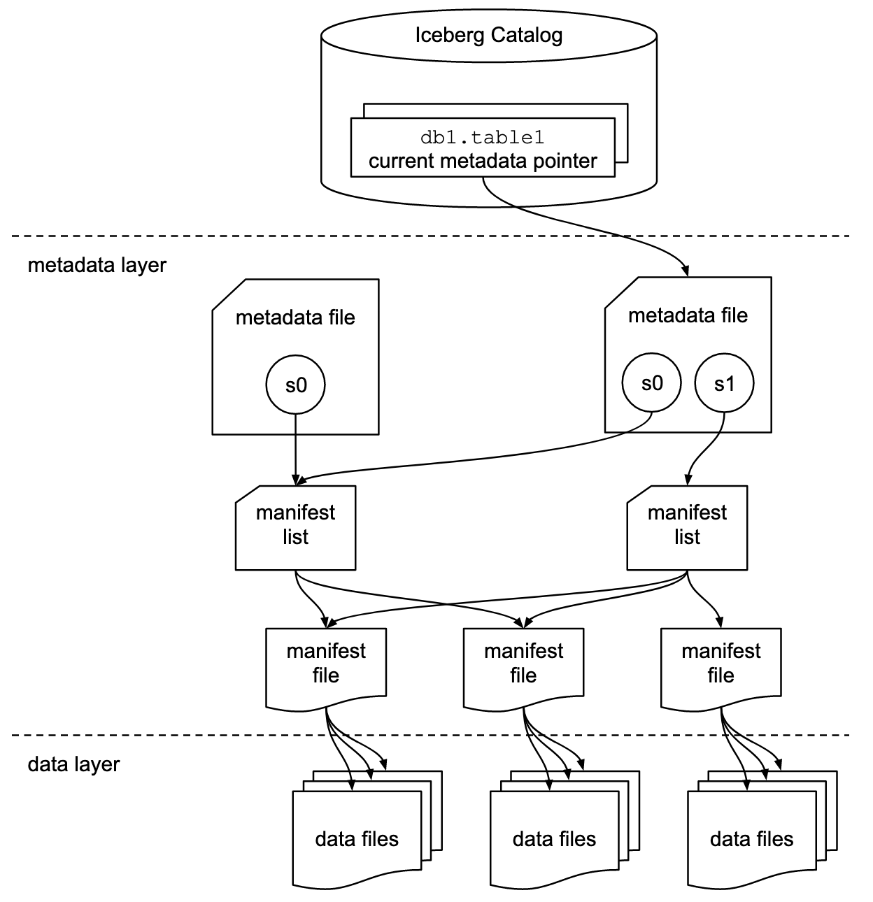
Starting from the bottom are your data files in the data layer. These are the files in your storage layer, such as objects stored in Amazon S3. Iceberg is a table format, however it is expecting Apache Parquet files compressed using Zstandard (ZSTD, developed by Facebook) by default. It does support ORC and Apache Avro. Going in order from above the data files are:
- Manifest Files: The manifest file contains a manifest of the paths leading to related data files which contain columnar lower and upper boundaries for the fields within them. This greatly aids in the performance of the query plan as files outside of a given bound are automatically pruned – which is to say ignored, not deleted.
- Manifest List: The manifest list contains entries of the manifest files that pertain to a given snapshot, which is a point-in-time complete description of a table’s schema, partition, and file information. Like the manifest file itself, the manifest list contains important metadata, such as partitioning statistics and data file counts. The partitioning statistics are also used to selectively prune non-pertinent manifest files as part of query planning. For instance, if you wanted to search for partitions between April and October in 2023, the manifest list will contain information about which manifest files pertain to those date ranges.
- (Snapshot) Metadata File: This file contains information about each snapshot of the table which includes the paths to the various manifest lists, current schema, and partitioning specification. This is typically written as an Apache Avro file type.
- Database and Table: This is standard fare in AWS Glue. A database is a collection of tables, and a table defines the top level path to the files for your Iceberg table. For instance s3://my-cool-lake/iceberg/some_log_source/. Importantly, AWS Glue Data Catalog does not track partition information as it does for standard Glue tables.
- Catalog: While Iceberg does support many different metadata management tooling, when using Amazon Athena for Iceberg, you must use AWS Glue: so in this case the catalog is AWS Glue Data Catalog. There is no escape!
Nine Benefits of Iceberg (on Amazon Athena)
- Transparency – One of the best benefits of Iceberg on AWS Glue Data Catalog is that it is mostly transparent, meaning there is no difference between querying an Iceberg table and a standard Glue table. SecDataOps teams writing analytics and detection content against the tables using Spark DataFrames or SQL would not need to change anything.
- ACID Compliance – Beyond that, there are more technical benefits to using Iceberg. As noted before, Iceberg tables have full ACID compliance – Atomicity, Consistency, Isolation, and Durability – and this is encapsulated in snapshots. Not only are snapshots a point-in-time record of a table, but also a pattern that guarantees isolated reads and writes. Detections and business intelligence (BI) dashboards reading the table will always have a consistent version, while data engineering pipelines will only ever perform metadata swaps after new data is done writing, as needed.
- Isolated Reads and Writes – There is no need for locking to enforce isolation (or to “trick” a user into isolation via blocking). Changes are made in a single atomic commit after all operations are completed. The snapshots provide durability and disaster recovery. They are tracked within the manifest files, you can rollback to a snapshot, go back to the current snapshot, and merge between them as required. If a data entry or configuration error causes a change in a column name, or adds an extra column, you can simply move to another snapshot for other live jobs (such as detections) while you correct the error.
- Schema Evolution – When you are done reconfiguring the pipelines, you can delete the snapshot and its subsequent metadata and data layer, and not interrupt operations. This isn’t solely a disaster recovery or error correction feature. Snapshots are created to execute on, and arguably the most compelling reason to adopt Iceberg: schema evolution. As your SecDataOps practice matures, you will find yourself wanting more data but also wanting to change what you have.
Want to migrate in-place to OCSF from another data model? You can do that with Iceberg. Want to include some extra columns needed to write more accurate and fine-grained detections? Want to store aggregates in columns alongside the data? Found out you don’t need some data tables? Want to simply rename columns? You can do all of that thanks to the snapshots.
- Fine-grain partitioning – Due to the predicate pushdown and pruning of files in the metadata and data layers, using finer-grained partitioning is back in play. Using Hive or AWS Glue Data Catalog for non-Iceberg tables is issue-prone. The catalog itself became a bottleneck, as it was the arbiter and gatekeeper of all metadata, resulting in having to spend time scanning non-pertinent partitions and files within your storage as it built the query plan.
- Hidden partitioning – Harkening back to schema evolution, you can likewise evolve your partitioning if you started without any partitions or with a wider timeframe in your partitions. Iceberg uses hidden partitioning, which does not require the partitions being stored as a column name in your table (which is why AWS Glue doesn’t collect this information), which allows for the flexibility of changing partitions in Iceberg.
Note: While Iceberg supports changing the partitions, Amazon Athena does not, due to Iceberg’s hidden partitioning.
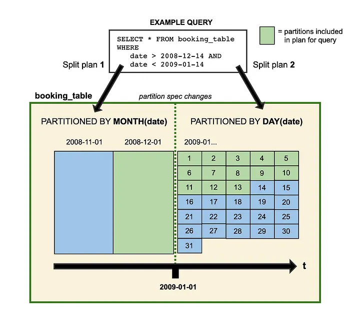
- Split-planning – Iceberg uses split-planning with queries so your old data that was partitioned by month can co-exist with newly added data that is partitioned by day. It does this by executing the first query plan against the older schema specification and then the new specification, and combining the files (FIG. 2). As partitioning changes happen in metadata, Iceberg will not go out of its way to rewrite files, and, since the manifests keep track of where the data files are and how they pertain to snapshots, the new datetime (or timestamp) truncation and filtering can be applied to both specifications transparently.
- Compaction management – When using Iceberg, you are not suddenly immune from the “small file problems” which plagues many data lakes. Due care still needs to be taken to attempt to use batch workloads to write data as densely as possible, or compaction operations need to run as part of the Ops piece of your SecDataOps team. Fortunately, Iceberg provides SQL commands of OPTIMIZE and VACUUM which allow data files to be rewritten into bigger files and for snapshots that exceed a given time period and/or orphaned data files to be removed, respectively.
These are three huge data engineering operational undertakings that can be solved with SQL Data Manipulation Language (DML) statements. However, that does not totally absolve your SecDataOps team of its Ops burden. These are whole-table operations and should be used from the start and on a scheduled time with predicates to avoid cost overruns and performance degradation.
Note: Iceberg has several OPTIMIZE strategies, however, Amazon Athena only supports BIN_PACK which rewrites the smaller files into larger files.
- Adding (not duplicating) data – Iceberg allows you to add data in place with SQL statements INSERT INTO and MERGE INTO. The first command allows you to append data into the table that matches the same schema. This is a powerful command (albeit potentially very slow and expensive) that can be useful to quickly migrate a Glue table into Iceberg in place. The latter command allows you to perform “upserts” into the table. This is useful where there are records in certain tables you would rather update than create a duplicate entry for, such as updating security findings from a CSPM or vulnerability management tool.
When using regular AWS Glue tables, you either need to execute SQL statements with Athena or re-run a Glue crawler to update the metadata in the Glue Data Catalog as necessary. This requires ensuring your writes into Amazon S3 have completed and the schema stays the same before running the crawler. Only when the data is logged into the catalog will your queries and BI reports incorporate this new data.
It is important to note that while INSERT INTO and MERGE INTO are great for sub-terabyte tables and small writes, it is much more efficient to use a framework, such as PySpark or AWS Data Wrangler, to append and merge data into Iceberg. As of the publication of this blog, Glue crawlers do support Apache Iceberg tables within Glue, so that option does exist.
But, Does Your Team Need Iceberg?
That said, your SecDataOps team may be more mature in its practices and adoption of data lakes and supporting technologies and may not have the same churn and evolving demands as other, newer teams. If you have simplistic, Write Once Read Many (WORM) workloads with very low (if any) demand to evolve schemas or partitions, do not have datasets that can grow to several dozen terabytes if not petabytes, or do not have the skills to operationally maintain Iceberg – you do not need it.
Iceberg is a great technology. However, it is not one that instantly makes your query performance faster, costs cheaper, or lets your SecDataOps team do its job any better. If you do not require ACID compliance, and are already invested in enterprise data warehouses such as Snowflake, Google BigQuery, or Oracle Autonomous Warehouse, you likely do not need to adopt the table format.
Note: At the time of this publication, Snowflake has started to release support for the Iceberg table format within their platform.
Even if you will not be implementing Iceberg right away, there is value in learning how to use it. In the next section, you will use Python, AWS Glue crawlers, and SQL DML and DDL statements in Amazon Athena to generate synthetic data, catalog it in Glue, and insert it into a new Iceberg table.
Building an Iceberg Table
Building an Iceberg table in Amazon Athena is very simple. It does not differ much from creating a table using SQL in normal Glue tables.
Before starting, ensure you have followed the prerequisites in the Getting Started section of the Amazon Athena User Guide. Amazon Athena stores the results of queries in an Amazon S3 bucket in the same Region where you use Athena. You must have this setup to run queries and have the proper IAM permissions to use the Athena service.
Additionally, you will need to create another Amazon S3 bucket in the same Region that will be used as the data lake storage. You should have IAM permissions to write and read from the bucket as well as access to AWS Glue APIs to run a crawler against the data.
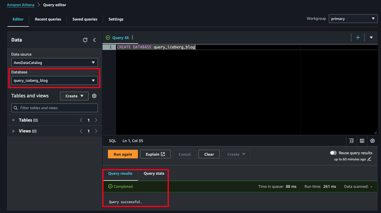
Step 1: Create a new Glue database. A database is a logical collection of Glue tables, no matter what the table format is. Colloquially, Glue and Athena are used interchangeably when referring to the databases or tables, but they are created in the Glue Data Catalog. If you change the name of the database, ensure you change it for all other relevant SQL commands in this blog. From the Athena query editor, execute the following statement.
CREATE DATABASE query_iceberg_blogIf successful, you will receive a Completed: Query successful message in the Athena console as shown below (FIG. 3). In the data selector, select the new database, and you will see there are not any tables or views created yet (also shown in FIG. 3).
Step 2: Create the actual Iceberg table. Athena creates Iceberg v2 tables using the CREATE TABLE command, not CREATE EXTERNAL TABLE. You will need to provide a LOCATION which is your S3 path and then specify the table type in TBLPROPERTIES. In the below query, ensure that you change the value of the S3 bucket and path to one that you will be using.
CREATE TABLE icy_ubuntu_ftp_logs (unix_time timestamp, operation string, response_code bigint, client_ip string, file_path string, size bigint, username string, message string)

LOCATION 's3://query-demo-iceberg-bucket/iceberg/ftp_logs/'

TBLPROPERTIES ( 'table_type' = 'ICEBERG', 'format' = 'parquet', 'write_compression' = 'ZSTD' )
Step 3: Execute the statement below – replacing your bucket name and path – without any other modifications. As before, if you do not have any issues you will receive a Completed: Query successful message in the Athena console. Errors can be introduced with invalid data types, SQL syntax errors (such as spacing out the table schema definition or adding newlines), and invalid table properties.
This SQL statement is telling Athena to create a new table named icy_ubuntu_ftp_logs. You create several fields with the syntax of <field_name> <data_type> and set a LOCATION of your S3 path where Iceberg will manage the data and metadata layer.
Step 4: Define the Iceberg table in TBLPROPERTIES. This is also where you can note what file format and compression is used. Iceberg tables created with Amazon Athena default to ZSTD-compressed Parquet files, but for the sake of the demo these are written out in case you wish to change them.
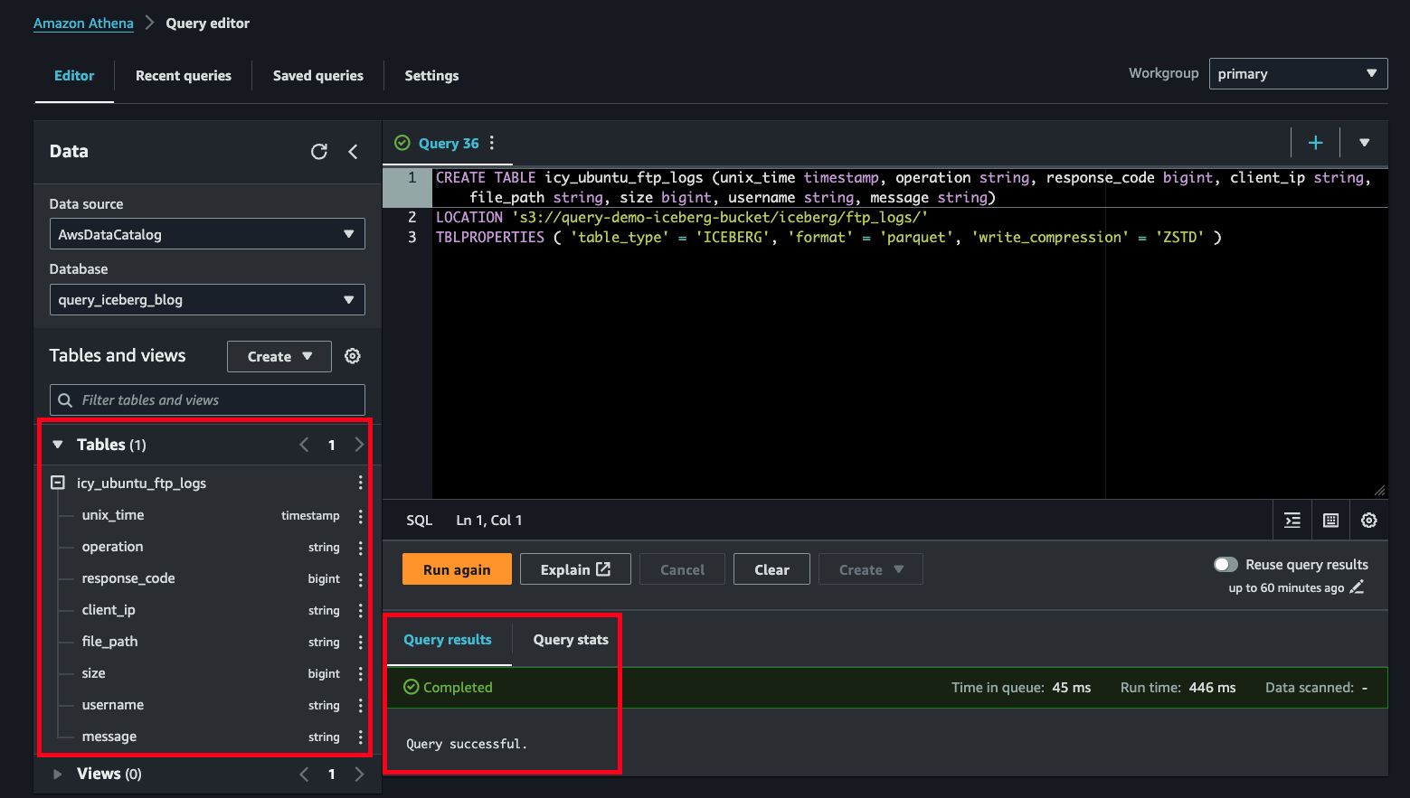
You can expand the newly created table in the data explorer in the Athena console to confirm the field names and data types as shown below (FIG. 4).
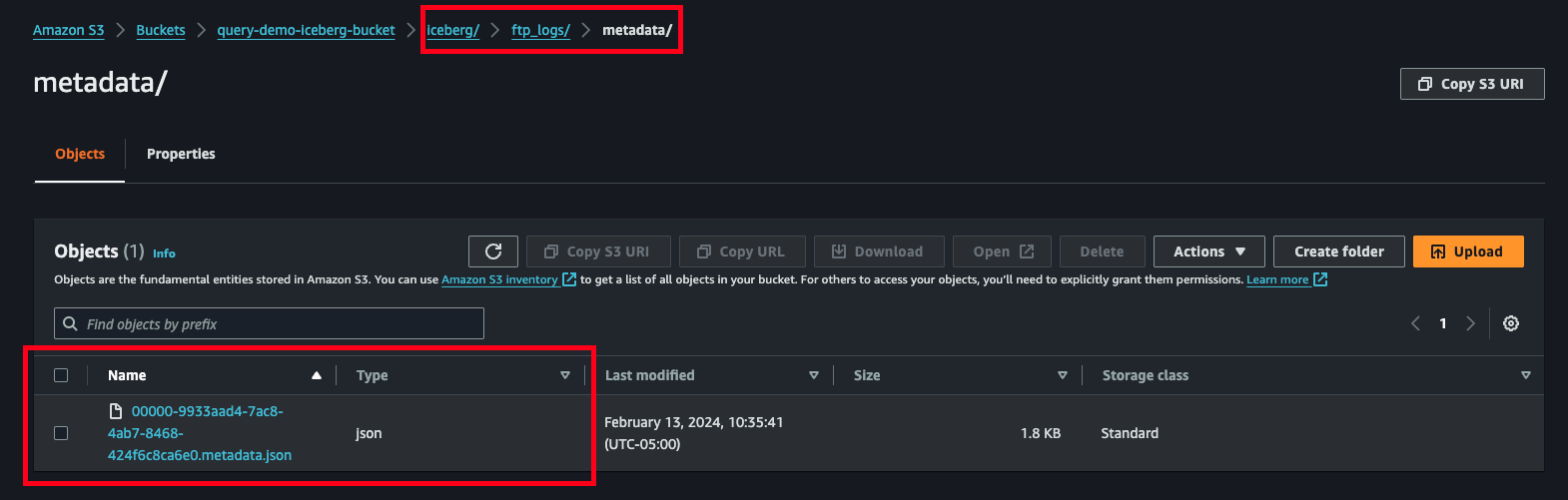
If you navigate to your S3 Bucket in the console, you can see the beginning of where Iceberg lays down its metadata layer and creates the first snapshot metadata file as shown below (FIG. 5). As you add data into your table and change the schema, this metadata layer will continue to expand. This all happens automatically and does not need any input from the user outside of planning the usage of OPTIMIZE and VACUUM statements.
Congratulations, you have an Iceberg table! But it is not much use without any data in it. While you can load Iceberg with frameworks such as Spark, that may be too heavy-handed for a quick demo. The quickest way to add data is to use the INSERT INTO command in a SQL statement and provide data in-line. Use the following SQL to insert some synthetic data into your table. Notice we are using the CAST command to translate a datetime to a timestamp type in Glue Data Catalog for our table.
INSERT INTO icy_ubuntu_ftp_logs (unix_time, operation, response_code, client_ip, file_path, size, username, message)
VALUES
(CAST('2024-01-25 10:23:49.000000' AS timestamp), 'RMD', 250, '64:ff9b:0:0:0:0:34db:6b1a', '/home/webuser/public/contoso.org/secure/query.toml', 0, 'root', 'Directory removed successfully.'),
(CAST('2024-01-25 08:53:19.000000' AS timestamp), 'LIST', 550, '64:ff9b:0:0:0:0:34db:6b1a', '/home/user/ftp/emails.txt', 0, 'guest', 'Failed to list directory. Directory not found'),
(CAST('2024-02-13 10:23:49.000000' AS timestamp), 'STOR', 550, '192.241.239.40', '/home/webuser/public/widget.co/public/signups.conf', 408371, 'administrator', 'Failed to upload file. File unavailable or access denied.'),
(CAST('2024-02-07 07:13:59.000000' AS timestamp), 'LIST', 550, '10.100.2.63', '/home/user/ftp/homepage.csv', 0, 'root', 'Failed to list directory. Directory not found.'),
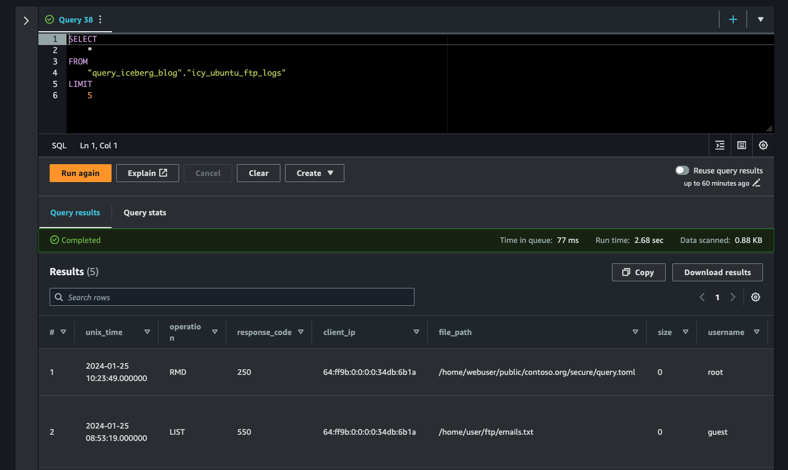
(CAST('2024-02-01 11:49:47.000000' AS timestamp), 'MKD', 550, '64:ff9b:0:0:0:0:a64:b1', '/var/vsftpd/emails.xslx', 0, 'root', 'Failed to create directory. Directory already exists.')As before, if your query succeeds you will get another Completed: Query successful prompt in Athena. Execute another SQL statement to see the results within Iceberg. The SELECT command is where you would select the specific fields in your table to display back, typically using predicates which are defined in the WHERE statement (not shown) to further conditionalize your SQL statements. SELECT * returns every field and record (columns and rows) and the LIMIT statement is used to define the total number of rows brought back. In your case, there are only 5 records in the table to begin with.
SELECT

    *

FROM

    "query_iceberg_blog"."icy_ubuntu_ftp_logs"

LIMIT

    5
In Athena, you will receive your results back in a columnar format, much like you would in a real relational database table of structured and semi-structured data as shown below (FIG. 6).
Now, while you can parameterize INSERT INTO queries and automate executing them using Boto3 and the Athena APIs, that is highly inefficient and will most likely lead to throttling and data loss. In the next section you will use a Python script to generate synthetic data, create a Glue table the traditional way with a Glue crawler and migrate that data into Iceberg.
Generating and Migrating Data to Iceberg
In this section you will use a Python script to generate synthetic data representative of preprocessed FTP logs from a Debian-based Linux system such as Ubuntu. You will use the AWS CLI to upload the data, create, and start a Glue crawler to create a Glue table and use more SQL statements to migrate the data to your Iceberg table and modify certain properties.
- Firstly, ensure you have the AWS CLI installed and configured on your system, and you have the proper IAM permissions to upload objects to Amazon S3, and to create and run crawlers in AWS Glue. The Python script is available from Query’s blog code GitHub, here. If you would rather skip running the script and only use the data, you can get it in JSON here and in ZSTD-compress Parquet here.
- Create a new directory for the demo data, instantiate a Python virtual environment and then execute the script with the following commands. Modify them for your operating system. These commands were executed on a MacOS. If you do not have Brew installed, refer here.
brew install python3

brew install wget

mkdir ~/Documents/query_iceberg_demo

cd ~/Documents/query_iceberg_demo

wget https://raw.githubusercontent.com/query-ai/blog-code/main/samples/Amazon%20Athena%20and%20Apache%20Iceberg%20for%20your%20SecDataOps%20Journey/python/synthetic_ftp.py

pip3 install virtualenv

virtualenv -p python3 .

source ./bin/activate

pip3 install pandas

python3 synthetic_ftp.py
The Python script will create 15000 synthetic JSON logs (such as the example below and what you inserted in your Iceberg table) and write them into a ZSTD-compressed Parquet file. If you had changed the file properties or compression scheme within TBLPROPERTIES when you first created your Iceberg table, modify the Python script to write the Pandas DataFrame to the proper file format with the correct compression.
{

        "unix_time": 1705287749,

        "operation": "MKD",

        "response_code": 257,

        "client_ip": "2600:1f18:4a3:6902:9df1:2d37:68ce:e611",

        "file_path": "/var/www/html/board_minutes.pptx",

        "size": 0,

        "username": "info",

        "message": "Directory created successfully."

 }
If you want to account for a larger time range of synthetic dates being generated, modify the generateSyntheticTimestampNtz() function within the script and change the first datetime values within the randTs variable, as shown below.
def generateSyntheticTimestampNtz() -> Tuple[int, str]:

    """

  Generates a random TIMESTAMP_NTZ formatted time and Epochseconds.

  """

    randTs = random.randint(

        int(datetime.datetime(2024, 1, 1).timestamp()),

        int(datetime.datetime.now().timestamp())

)- After running the script, upload the Parquet file into S3 with the following command. Ensure you change the name of the S3 Bucket. If you modified the script to create multiple files, you can upload your entire local directory as well.
aws s3 cp synthetic_ftp_logs.parquet.zstd s3://query-demo-iceberg-bucket/raw/ftp/- Next, use the CLI to create and execute a Glue crawler. If you have never used a crawler, refer to the Tutorial: Adding an AWS Glue crawler section of the AWS Glue User Guide and at least create an IAM Service Role for Glue. This is what gives Glue the permissions to read and write objects to and from your S3 buckets, ensuring you give it permission to access your particular S3 bucket.
- Once complete, or if you have an existing role, replace it with the below placeholder value in the –role argument. Additionally, ensure that the value for –database matches what you named your Glue database in the first command you ran in this blog. You will need iam:PassRole permissions to create the crawler and attach your Service Role, too.
aws glue create-crawler \

    --name query_iceberg_demo_crawler \

    --role arn:aws:iam::111122223333:role/service-role/AWSGlueServiceRole-CrawlS3 \

    --database-name query_iceberg_blog \

    --targets '{"S3Targets":[{"Path":"s3://query-demo-iceberg-bucket/raw/ftp/"}]}'
Provided you do not encounter any errors, run the crawler manually. This will cause the crawler to look at all the Parquet file(s) in your path and introspect the schema and data within it and log them in the Glue Data Catalog. Typically, this process takes up to two minutes to run, but can vary depending on how much data you generated.
aws glue start-crawler --name query_iceberg_demo_crawler- Once you’ve waited enough you can check the console or use the other command below to ensure that a table was created. For example, my crawler ran successfully and the TablesCreated value is 1.
aws glue get-crawler-metrics --crawler-name-list query_iceberg_demo_crawler
{
"CrawlerMetricsList": [
{
"CrawlerName": "query_iceberg_demo_crawler",
"TimeLeftSeconds": 0.0,
"StillEstimating": false,
"LastRuntimeSeconds": 53.505,
"MedianRuntimeSeconds": 53.505,
"TablesCreated": 1,
"TablesUpdated": 0,
"TablesDeleted": 0
}
]
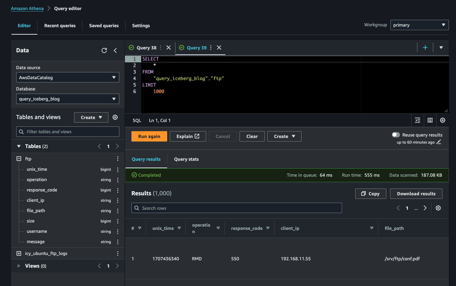
}Going back to the Amazon Athena query editor, execute the following SQL statement to verify that the data is in your Glue table. Your table should be named ftp, however, change the command in case you modified your path.
SELECT

    *

FROM

    "query_iceberg_blog"."ftp"

LIMIT

    1000
If successful, you should receive results back as shown below (FIG. 7). Take note that the unix_time column is in Epoch seconds (Unix seconds) which needs to be converted. When you migrate this data, we will use built in Athena DML commands to modify this, similar to how you did when running the first INSERT INTO command against your Iceberg table.
- To migrate data from an existing Glue table, view, or another Iceberg table, we can modify the INSERT INTO command to SELECT fields from another table to perform the insertion. This will allow you to append data that matches your schema into your Iceberg table. For this command to succeed you need to convert the Epoch seconds into a timestamp.
For this you use the from_unixtime() SQL function. For cases where you were writing Epoch milliseconds, Epoch microseconds, or Epoch nanoseconds, you would need to divide by the thousands of specific seconds. For instance, if you created the Epoch seconds from 6 digits of precision, the command would be from_unixtime(unix_time / 1000000000). As long as the rest of the data types match the destination data type, you can execute this statement without issue.
INSERT INTO

    icy_ubuntu_ftp_logs

SELECT

    from_unixtime(unix_time) as unix_time,

    operation,

    response_code,

    client_ip,

    file_path,

    size,

    username,

    message

FROM ftp
As usual, you will receive a Completed: Query successful message if the statement is executed properly. To confirm the changes, execute the following query to ensure that all the data was appended as expected into your Iceberg table.
SELECT * FROM "query_iceberg_blog"."icy_ubuntu_ftp_logs" LIMIT 750For more specific information from the table, you can use a WHERE clause to specify predicates within the statement. In this case, you can select specific IPs that would be generated in the logs where the response_code value is not 550. Mastering predicates, operators, and functions within SQL is crucial for effective security analysis, threat hunting, detection content engineering, and BI reports.
SELECT

    unix_time,

    operation,

    message,

    client_ip,

    file_path

FROM

    "query_iceberg_blog"."icy_ubuntu_ftp_logs"

WHERE

    client_ip in ('5.78.89.3', '37.221.173.241')

AND

    response_code != 550
As noted earlier, AWS Glue does not support adding partitions for Iceberg tables. The table you created is not partitioned. If you wished to create partitions, you would need to build another table and use INSERT INTO. Reach out to athena-feedback@amazon.com (along with the rest of the community) to have their product managers prioritize this quality of life feature.
In this section, you learned how to generate synthetic logs, upload them to S3 and index them in the Glue Data Catalog with a crawler. You also learned how to migrate this data into Iceberg using the INSERT INTO command and learned how to use basic predicates and operators to search for specific information in the logs. In the next section you will learn how to manipulate the Iceberg table and use built-in information within the Iceberg table format before cleaning everything up.
Working With Iceberg Tables
There is still more to be done with Iceberg, such as modifying column names, and working with the table metadata and the optimization commands. When we inserted the data into the table, we named the timestamp field unix_time to match the raw Glue table which stored the data into Epoch seconds. This can be confusing for team members interacting with the table, so we can quickly rename this column with Athena. We will use the ALTER TABLE DDL statement to change the column.
ALTER TABLE

icy_ubuntu_ftp_logs

CHANGE COLUMN

unix_time log_timestamp timestamp
If successful you will see the column name change immediately. The syntax of CHANGE COLUMN is <old_column_name> <new_column_name> <data_type>. You can issue yet another command if you want to change client_ip to source_ip instead. As your detection needs or analysis requirements evolve, it can be helpful to standardize and normalize naming conventions, casing, and data types depending on the actual data in the field (FIG. 8).
ALTER TABLE

icy_ubuntu_ftp_logs

CHANGE COLUMN

client_ip source_ip string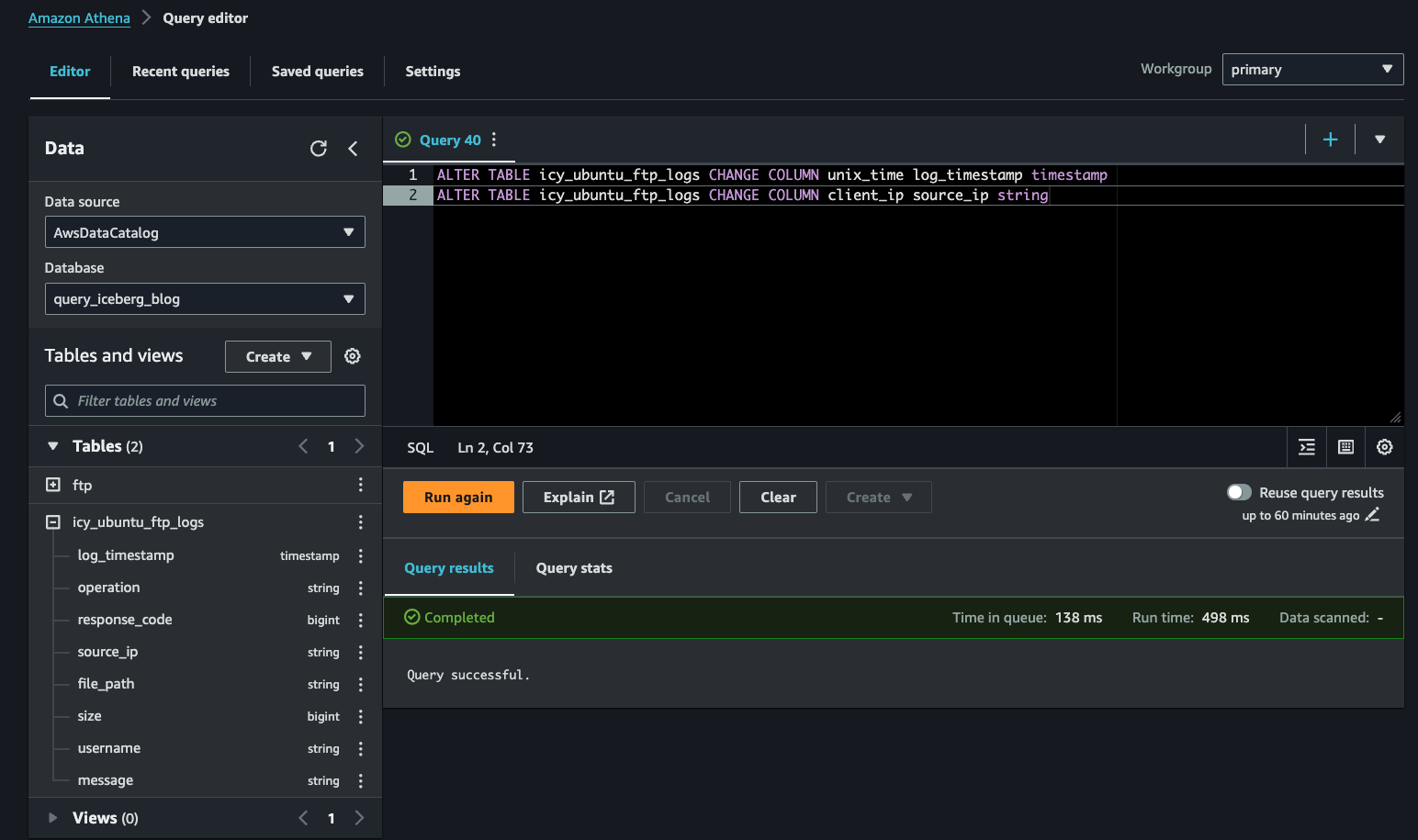
On top of changing the column names, you can also replace data in-place within the Iceberg table. This can be useful if you are logging pertinent data that can change, such as a computer hostname, a user’s primary email, the geolocation coordinates of a facility, or in this case swap IPv6 into their IPv4 version. In this (really bad) example, consider if you found out that the IPv6 address 2600:1f16:127a:2000:c802:a75f:63f1:f9c9 which belongs to AWS’ us-east-2 Region IPv6 space actually corresponds to 18.217.82.104? You can easily replace that value within Iceberg using the UPDATE command which combines INSERT INTO and DELETE.
UPDATE icy_ubuntu_ftp_logs

SET source_ip = '8.217.82.104'

WHERE source_ip = '2600:1f16:127a:2000:c802:a75f:63f1:f9c9'
The UPDATE command specifies a table. SET takes a column (field) name and an equals operator for whatever value you want to change the column value to. The WHERE predicate is your conditional statement. Note: you must have the same data type when issuing this UPDATE command.
To confirm that the update took place, attempt to search for the old IPv6 address in the table with the following command. You should not receive any results after executing the SQL statement.
UPDATE icy_ubuntu_ftp_logs

SET source_ip = '8.217.82.104'

WHERE source_ip = '2600:1f16:127a:2000:c802:a75f:63f1:f9c9'
All of this data manipulation may make data governance personnel faint, as well as security personnel depending on the data in the table. How do you audit it? Iceberg has several dedicated metadata properties per table that allows you to inspect the associated files stored in S3, the manifest files in the metadata layer, the query history and changes of a table, the available partitions, and the snapshots. You can query these facts with simple SQL statements in Athena as shown below. These statements lend themselves well to automating, as part of audit activity and tracing breaking changes.
SELECT * FROM "table$files"
SELECT * FROM "table$manifests"
SELECT * FROM "table$history"
SELECT * FROM "table$partitions"
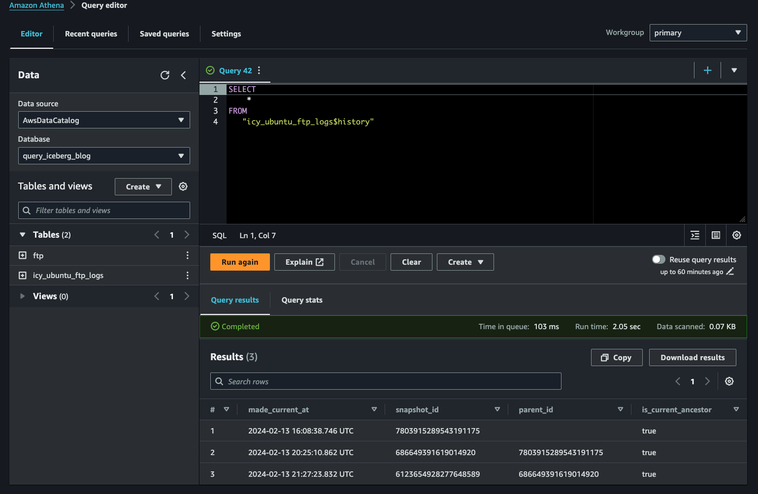
SELECT * FROM "table$snapshots"To review all of our changes thus far, check the $history metadata with the following command. Note the usage of double quotes around the table name and metadata informational decorator.
SELECT

    *

FROM

   "icy_ubuntu_ftp_logs$history"
The result of this statement will provide you with the Iceberg snapshot identifiers, which can be used for the time travel and rollback functionality of Iceberg. The first entry, the snapshot_id without a paired parent_id, is the first version of the table’s schema. You then made changes to the column names which are also captured in the next two snapshots. This history is not a replacement for an audit log. You would need to use CloudTrail (if you’re using Athena) to determine the specific AWS IAM principals (e.g., federated identities, IAM Users, etc.) taking specific actions against the table (FIG. 9).
If you want to get specific information on the snapshots, such as an overview of what changes went into it (changed partitions, added records, changing file sizes), execute the following statement and refer below (FIG. 10) for example results.
SELECT

    snapshot_id,

    summary

FROM

    "icy_ubuntu_ftp_logs$snapshots"
To revert the table back to its original state, you can use the snapshot_id with the special FOR VERSION AS OF predicate within your SQL statement. Replace the value of the snapshot identifier with your own from the $history or $snapshots metadata.
SELECT

    *

FROM

    icy_ubuntu_ftp_logs

FOR VERSION AS OF 7803915289543191175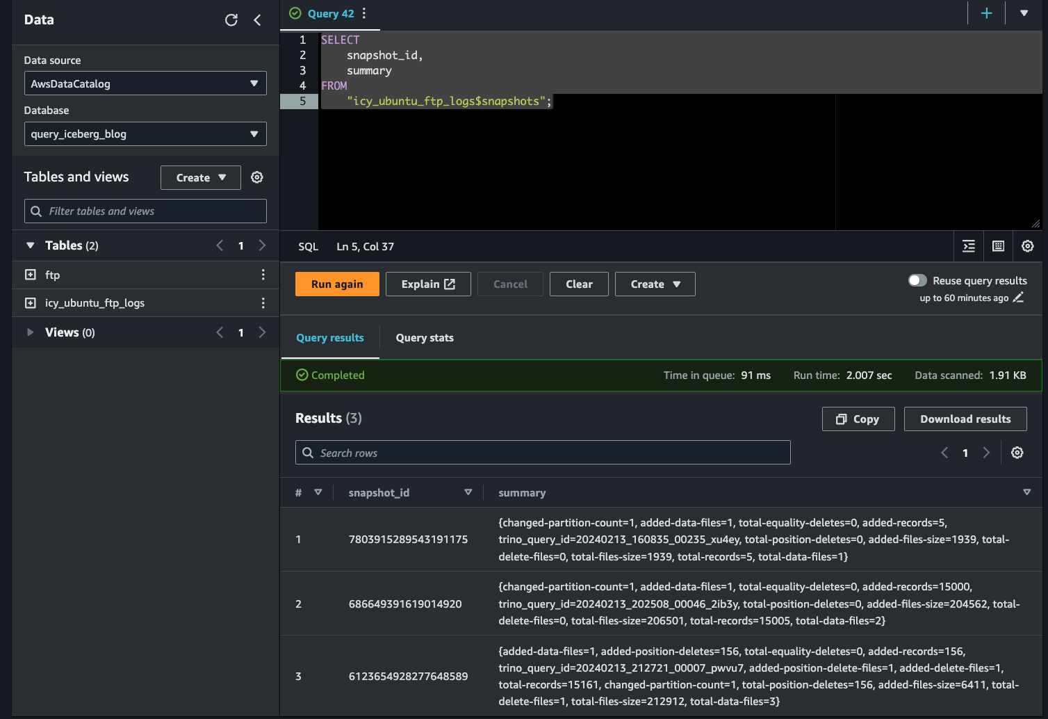
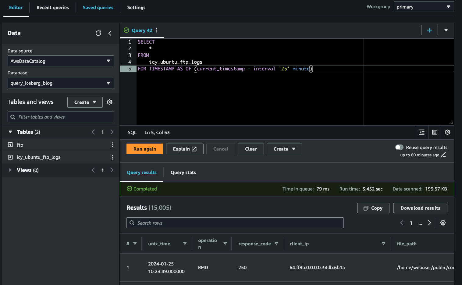
You will receive results back from the original INSERT INTO command which only had five records and had the original unix_time and client_ip column names. Another term that is nearly ubiquitous with Apache Iceberg is “time travel.” Using another specialized predicate FOR TIMESTAMP AS OF, you can simply query the table as of a specific timestamp without the need for a snapshot ID. Change the interval based on how long you have taken between steps and you may get different results, especially from the UPDATE command changing the IPv6 to an IPv4 address.
SELECT

    *

FROM

    icy_ubuntu_ftp_logs

FOR TIMESTAMP AS OF (current_timestamp - interval '25' minute)
In my example, the time travel worked to see the table before changing any column names or the value within them, as shown below (FIG. 11).
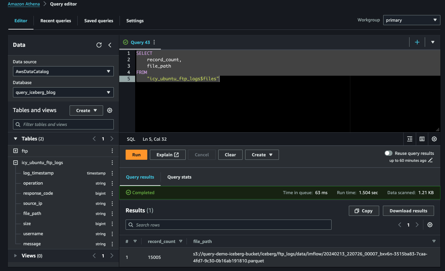
Finally, you can use the OPTIMIZE command to reduce the smaller files and reconsolidate them. Remember, you should run this command on a schedule when using Glue Data Catalog due to the fact that Athena only supports BIN_PACK as the optimization strategy. First, review how many files there are by using the $files table metadata.
SELECT

    record_count,

    file_path

FROM

    "icy_ubuntu_ftp_logs$files"
Now, execute the OPTIMIZE statement and follow up with repeating the above query. You may need to generate more synthetic data and INSERT INTO your Iceberg table to see a noticeable difference.
OPTIMIZE icy_ubuntu_ftp_logs REWRITE DATA USING BIN_PACKI was able to consolidate down to a single file path with all 15005 records within it, as shown below (FIG. 12).
This concludes the Iceberg content for this blog. To tear down the resources that you created, execute the following SQL statements to delete both tables and then the database. Modify the values as necessary.
DROP TABLE ftp

DROP TABLE icy_ubuntu_ftp_logs

DROP DATABASE query_iceberg_blog

Lastly, delete the Glue crawler using the AWS CLI.

aws glue delete-crawler --name query_iceberg_demo_crawler
In this section you learned more about working with the specialized features of Apache Iceberg. You learned how to change table columns, as well as their data, selectively. You learned how to audit the various metadata of a table, such as its change history, related files, and snapshots. You learned how to use snapshot-based reversion as well as Iceberg’s time travel to view different versions of the table at various times. Finally, you learned how to delete your resources. You will need to remove the data from S3 or delete the bucket outright to avoid accruing any potential costs.
Conclusion
Iceberg helps to solve for the maturing data needs of a burgeoning SecDataOps team by allowing you to evolve the schema and (soon hopefully) evolve the partitioning of tables. Your teams can migrate current Glue tables into Iceberg, and, if changes are made, can alter their tables and travel through time to rollback to stable points. Additionally, SecDataOps teams can make use of hidden partitioning (though, they cannot change them) and the `OPTIMIZE` and `VACUUM` commands to maintain performance.
Of course there is always more to say and more to do with Apache Iceberg. In the next entry we will explore the use of AWS Data Wrangler to easily append and grow our Iceberg tables, use more advanced SQL, and lean more heavily into Iceberg features and functionality as appropriate.
The Query Federated Search Platform already has an integration with Amazon Athena to search data indexed by the AWS Glue Data Catalog, including Glue tables and Iceberg tables. If you want to search high volumes and a variety of security and security-relevant data, but do not want to memorize yards worth of SQL statements, contact Query.
Until then…
Stay Dangerous.