
Partitioning your data is one of the most important things you can do to improve the query performance of your data lake in Amazon S3. When building tables in AWS Glue Data Catalog and querying with Amazon Athena, as your data volumes grow, so do your query wait times.
In this blog you will learn how to use Jupyter notebooks running on Amazon Elastic MapReduce (EMR) Serverless Workspaces and PySpark to quickly apply time-based partitions to your data where none exist. You will also learn how to generate synthetic data to test with and benchmark partition performance yourself.
This blog is long, so here are a few shortcut links if you know what you’re looking for:
- Unpartitioned Security Data Problems
- PySpark & Amazon Elastic MapReduce Overview
- Generate Synthetic Data
- Benchmarking Non-Partitioned Performance
- Auto-Partition Data with PySpark
- Querying Partitioned Tables
Unpartitioned Security Data Problems
The problems with unpartitioned data boil down to slower query performance and increased query costs. It is not uncommon for security data to be unpartitioned throughout any phase of the data lifecycle – be it raw data for an initial hydration of a data lake, or after it is normalized. Popular native forms of bulk data loading can also write data without partitions. For example, you can use Amazon Data Firehose or FluentBit to write data from APIs or hosts, respectively, and completely disregard dynamic partitioning with those tools.
When dispatching queries with Amazon Athena – or another query engine that interfaces with Glue Data Catalog – the metadata that underpins the tables (such as the file location) is retrieved from the catalog. Following that, each S3 object is scanned to look for the data that matches your SQL statement as part of the query execution.
For instance, you dispatch the following query against a table of Endpoint Detection & Response (EDR) telemetry named edr_telemetry.
SELECT

    agent_id,

    computername,

    ipv4_address

FROM

    "secops_database"."edr_telemetry"

WHERE

    first_seen_at > cast('2023-01-21 12:00:00.000000' as timestamp(6))
This query will retrieve the values of agent_id, computername, and ipv4_address fields from the edr_telemetry table where the timestamp for the first_seen_at field is greater than January 21st, 2023. Without a partition specified, your query engine will need to read the contents of every single file in your data lake to match the condition set in your WHERE clause.
For smaller tables with limited data, such as an asset inventory table, this query may still execute quickly. In my own benchmark, a table with 11 million rows of synthetic EDR data using that same query returned results within 45 seconds on average. Only your SecDataOps program can determine what “too long” is, but you should always seek to partition your data nonetheless.
In reality, if your team onboarded per-host EDR telemetry, such as data from Crowdstrike Falcon Data Replicator, these tables can easily get to 100s of millions – if not billions – of rows per year with only a few thousand endpoints. Likewise, collecting lower-level network logs from DNS resolvers or firewalls, network flows (such as Azure, GCP or AWS flow logs), or similar can always reach the same volume. Attempting to write a query as demonstrated above would likely either timeout or fail to execute altogether. If it did execute, it would take several minutes – if not hours – and likely cost several $100 USD per query.
When using the native Hive table format in AWS Glue Data Catalog, the path you write to S3 must match Hive-compliant syntax, meaning the partition has to follow the pattern of partition_name=partition_value such as year=2024. Without this, Glue crawlers (a popular mechanism for creating tables in Glue), will not automatically register these partitions. In addition to the naming convention, Glue partitions require location information which is the specific folder path for the data in S3 for a particular partition.
Not all is lost if you do not follow these conventions. If you create a table directly in Amazon Athena, you can use partition projection. With projection, Athena calculates partition values and locations using the table properties in Glue Data Catalog. The table properties allow Athena to ‘project’, or determine, the necessary partition information instead of having to do a more time-consuming metadata lookup in the Glue Data Catalog.
However, this method can prove complicated for teams lacking the SecDataOps expertise to continue to develop a partition project scheme. Additionally, this methodology only works for Amazon Athena, and using another query engine will ignore the projection completely. Likewise, the partition metadata is not trackable if you’re planning parameterized queries externally, using the DDL SHOW PARTITIONS query or using the Glue table API will not provide this information.
There is another way to quickly set partitions and create new external tables for your data, and that is using PySpark to dynamically set partitions based on a set (time-based) column and (re)write the data to Amazon S3. In the next section, you will learn about PySpark and how it is used within the AWS ecosystem before getting hands on with PySpark code.
PySpark & Amazon Elastic MapReduce Overview
Apache Spark and PySpark
PySpark is an interface for Apache Spark in Python that combines the simplicity and accessibility of Python programming with the power of the Apache Spark platform. Spark is a unified analytics engine designed for large-scale data processing with tools for batch processing, real-time streaming, machine learning, and graph processing. Spark operates by distributing data processing tasks across multiple compute nodes – such as across several Amazon EC2 instances, containers in Kubernetes, or otherwise – to achieve high performance and efficiency.
Spark’s resilience comes from its ability to handle failures and its optimization through advanced computational strategies like Directed Acyclic Graph (DAG) scheduling and in-memory processing. This makes it a preferred choice for processing big data and performing complex analytics. At its core, PySpark allows Python developers to leverage Spark’s API and its scalable data processing capabilities.
This means that tasks which traditionally required a lot of hardware and were complex to implement, such as analyzing large datasets or processing real-time data streams, can be accomplished more easily and with less code. One of the key features of PySpark is its ability to handle Resilient Distributed Datasets (RDDs), which are a fundamental data structure in Spark. However, for the scope of this blog, DataFrames are used instead of RDDs, because PySpark offers an API for DataFrames.
PySpark DataFrames are inspired by similar DataFrames such as those in Pandas and in R, but designed for scalability and efficiency in distributed computing environments. DataFrames in PySpark represent a collection of data distributed across the cluster, organized into named columns, similar to a table in Glue Data Catalog or a relational table in Spark SQL. This abstraction not only makes it easier for users to work with large datasets, but also optimizes performance through Spark’s Catalyst optimizer and Tungsten execution engine, which underpin execution plans and memory management, respectively.
For those new to PySpark, it’s worth noting that, despite its powerful capabilities, the learning curve can be steep. Understanding the basics of Python is essential, but it also helps to have exposure to single-node scripting using Pandas, especially in the context of moving to PySpark DataFrames. Though they are not truly one-to-one, and even with memory-optimized DataFrames such as those in Polars, there are differences in operators, methods, and usage to be aware of.
To get started with PySpark, one typically begins with setting up a Spark session, which is the entry point to programming with Spark. All operations are instantiated from the Spark session. For instance, the session is where DataFrames are created from, SQL is executed, Apache Parquet files are opened and read, data is appended into tables, and more. Additionally, the session is where configuration context is defined such as file or table-specific arguments, serialization, external libraries, environment variables, and more.
Within AWS, there are several ways to use Spark and PySpark, the most obvious being self-hosting containers or an entire Spark environment using Amazon EC2 or Amazon Elastic Container Service (ECS). While PySpark (and Spark by extension) is meant to run in multi-node clusters to distribute compute – you can operate Spark locally on a single machine to develop your scripts. This provides an easy-to-validate test bed for PySpark scripts or Jupyter notebooks that use PySpark APIs, and may be a way for SecDataOps engineers and analysts to jump straight into learning PySpark and bypass Pandas or Polars completely.
Amazon Elastic MapReduce (EMR)
The more popular way to run big data workloads – Spark, Apache Hive, Apache Hadoop, or otherwise – is using Amazon Elastic MapReduce (EMR). EMR is a big data solution to run large scale (sometimes multi-petabytes) data processing, interactive analysis, and/or machine learning workloads. As a platform service, EMR automates the deployment of software dependencies, cluster management, logging, encryption, and other operational tasks you would need to handle on your own when you self-manage a big data framework. Below (FIG. 1) is an AWS-produced high level graphic of EMR’s usage and deployment modes.
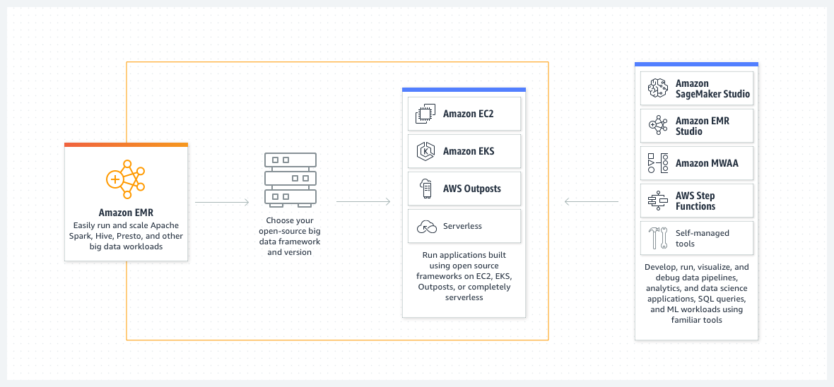
EMR has various modes of deployment, four to be exact, though you will only focus on the latest version for this blog.
- EMR-on-EC2: Standard mode of deployment that uses Amazon EC2 instances as its compute nodes
- EMR-on-Amazon Elastic Kubernetes Services (EKS): In this mode of deployment EMR can schedule and orchestrate big data runtimes on containers inside of an EKS Cluster.
- EMR-on-Outposts: AWS Outposts is a hybridized deployment where you can deploy AWS services on-premises in server racks, creating your own private cloud. Amazon EMR is a supported service for Outposts.
- EMR Serverless: In this mode of deployment, you eschew managing infrastructure and let AWS handle provisioning, scaling, and all other operations while you pick a big data framework to run jobs or interactive analyses on.
The Serverless deployment model optimizes against under- or over-provisioning and uses the exact amount of resources required to accomplish a job or analysis. This helps to also optimize costs, get started faster, and upper limits being set allow costs to be controlled in the case of a “runaway” job being scheduled.
About EMR Serverless
EMR Serverless packages the various big data frameworks and components into EMR Serverless release versions which correlate to pre-packaged frameworks and EMR Serverless-specific capabilities. For instance, EMR Serverless v6.15.0 packages Apache Spark v3.4.1, Apache Hive v3.1.3, Apache Tez v0.10.2, and allows for mutual-TLS connectivity between workers within (Py)Spark jobs. The release version and specific runtime (e.g., Hive, Spark, etc.) along with your Amazon Virtual Private Cloud (VPC) selection are specified in an EMR Serverless Application.
From your Application you can submit job runs, which are asynchronous tasks that run against a big data framework, such as HiveQL queries submitted to Hive or a PySpark script, to automatically partition data. Transparently, AWS handles the spawning of workers which are the distributed computing nodes that execute tasks from your jobs, use AWS Identity & Access Management (IAM) permissions to interact with AWS services, and more. Jobs can be submitted using the API, SDKs, the console, or you can use EMR Studio to do so.
EMR Studio is an Integrated Development Environment (IDE) where interactive analyses – such as Jupyter notebooks – and job runs can be scheduled from. EMR Studio can be configured for federated access initiated from an Identity Provider (IdP) such as Microsoft Entra ID, so SecDataOps engineers and analysts can access it without needing access to underlying AWS resources. You must use EMR Serverless release version v6.14.0 and above to specify an application as the compute backend for EMR Studio jobs and interactive workloads. It is automatically created for you when you create your first EMR Serverless Application.
In the next section you will prepare synthetic data to test the automatic partitioning of data using PySpark and upload it to Amazon S3.
Generate Synthetic Data
To provide a test bed for benchmarking performance of using partitions or not within your Amazon Athena SQL queries, as well as provide a mechanism to run the PySpark example against, you will first generate synthetic data. This data is based on a very simplified and generic subset of data you would expect from EDR telemetry, such as from Crowdstrike Falcon Data Replicator (FDR) or SentinelOne’s DeepVisibility functionality within the Singularity Platform. This type of data is used by SOC analysts and threat hunters alike to provide machine context to alerts generated from EDR tools and to hunt for specific tradecraft or behaviors on EDR-equipped endpoints and servers, respectively.
Before starting, ensure the following prerequisites are met:
- You have permission to interact with Amazon EMR Serverless, Amazon Athena, AWS Glue, AWS IAM, Amazon S3 in an AWS Account.
- You have set up Amazon Athena. If not, refer to the Getting Started section of the Amazon Athena User Guide.
- You have the AWS CLI configured, and Python version 3.9 or above (ideally >=3.11.4) installed locally.
- Accomplish all tasks within the Getting started with Amazon EMR Serverless section of the Amazon EMR Serverless User Guide.
In this section, you will generate as much synthetic data as you want to, upload it to S3, create an AWS Glue database, and finally create an AWS Glue crawler to crawl and index the data into a Glue table.
Step 1: Download Files
First, download the following files from our GitHub repository.
- synth_edr.py Python script, here.
- malicious_samples.json JSON file, here. This contains MD5 and SHA256 hashes of malware samples courtesy of theZoo GitHub repository.
- benign_samples.json JSON file, here. This contains MD5 and SHA256 hashes of several 100 random samples of files from the RDS_2021.12.2 SQLite database produced by the NIST National Software Reference Library (NSRL).
Step 2: Create New Directories and Instantiate a Python Virtual Environment
Second, create two new directories and instantiate a Python virtual environment to download some dependencies with. These commands were run on a MacBook Pro (Apple M1 Max/32GB) with macOS Ventura 13.5.1. Adapt them for your system as required.
mkdir ~/query_pyspark_blog

mkdir ~/query_pyspark_blog/edr_samples

cd ~/query_pyspark_blog

pip3 install virtualenv

virtualenv -p python3 .

source ./bin/activate
Step 3: Install Required Dependencies
Third, install the required dependencies not included in the Python core libraries. Faker is used to generate synthetic usernames and hostnames, and Pandas (and PyArrow) are used to create Zstandard-compressed Apache Parquet files. Parquet is a columnar binary file format that is very read-efficient (especially compared to JSON and CSV file formats), and Zstandard is a performant compression method developed by Facebook. Within data lakes and data lake houses, Zstandard-compressed Parquet could be considered the “golden standard”.
pip3 install pandas

pip3 install pyarrow

pip3 install faker
Step 4: Generate Synthetic EDR Data
Finally, use the Python script you downloaded earlier to generate synthetic EDR data that contains synthetic IP addresses, hostnames, usernames, file paths, file samples complete with MD5 and SHA256 hashes, and several other details found within raw EDR telemetry. There are several modifications you can make to the script to change the time range of generated logs, as well as the types of IP addresses generated.
To change the data range, modify the generateSyntheticTimestampNtz() function. This function starts by picking a random integer from generated timestamps between a date in the past (by default this is set to 10 JUNE 2023) and the current time. You can modify the second line to generate synthetic logs in the future, or you can lessen the data range by modifying the first line.
def generateSyntheticTimestampNtz() -> Tuple[int, str]:

         """

    Generates various random timestamps and datetimes

    """

        randTs = random.randint(

            int(datetime.datetime(2023, 6, 10).timestamp()),

            int(datetime.datetime.now().timestamp())

        )

  ## ...continued below...
To modify the types of IP addresses generated, modify the generateSyntheticRfc1918IpAddress() function. This function uses the ipaddress library to pick from several RFC1918 (private IP addresses) CIDR ranges and generate an IP address from there that does not include router or broadcast addresses. If any of these IP addresses overlap with your own internal ranges and you do not wish to have them included you can remove the CIDRs or change them to different ranges as shown below.
def generateSyntheticRfc1918IpAddress() -> str:

    """

    Generates a random IP address within a randomly selected CIDR range.

    """

    network = ipaddress.IPv4Network(

        random.choice(

            [

                "10.100.0.0/16","10.0.0.0/16","192.168.0.0/16","172.16.0.0/16"

            ]

        ),

        strict=False

    )

    ## ...continued below...
The Python script uses sys.argv to accept arguments when you run the script. The first argument is the number of batches of EDR logs you wish to generate, and the second argument is the amount of logs per batch. You can set this to any amount, but I recommend generating at least two million entries to ensure a more evenly distributed dataset. To generate that amount, run the following command:
python3 synth_edr.py 8 250000Step 5: Upload Synthetic Data to Amazon S3
Using the AWS CLI, copy the files from your file system to an Amazon S3 bucket you have permissions to read and write objects from. Later in this blog you will use PySpark to interact with it from Amazon EMR Serverless as well, so take note of the S3 path your upload to. Ensure you replace the name of the bucket with your own.
aws s3 cp ./edr_samples s3://query-demo-iceberg-bucket/synthetic_edr_demo_raw/ --recursiveNavigate to the query editor in the Amazon Athena console to create a database. In AWS Glue (which is what Amazon Athena uses by default as its metastore) a database is simply a logical collection of tables which are references to schemas and objects stored within Amazon S3. You can ultimately name the database whatever you want, just take note of it for creating the Glue crawler in the next step.
CREATE DATABASE pyspark_demo_dbNext, using the AWS CLI again, create a Glue crawler. Crawlers will read and introspect the schema – including the serialization, compression, data types, and column names – of data in provided S3 paths. From there, the Crawler creates a table using this introspection information within the database of your choosing. When you do not know the exact schema or relevant information for your data, this remains one of the fastest mechanisms available to SecDataOps engineers and analysts to quickly onboard data into a data lake or data lake house built on Amazon S3.
Note: If you have never used a crawler, refer to the Tutorial: Adding an AWS Glue crawler section of the AWS Glue User Guide and at least create an IAM Service Role for Glue. This is what gives Glue the permissions to read and write objects to and from your S3 buckets, ensuring you give it permission to access your particular S3 bucket.
Ensure that you modify the crawler name, the IAM Role ARN, the database name, and Amazon S3 bucket path as required before executing the following command. If there was not an error, you will likely not receive any feedback from the command.
aws glue create-crawler \

    --name query_pyspark_demo_crawler \

    --role arn:aws:iam::111122223333:role/service-role/AWSGlueServiceRole-CrawlS3 \

    --database-name pyspark_demo_db \

    --targets '{"S3Targets":[{"Path":"s3://query-demo-iceberg-bucket/synthetic_edr_demo_raw/"}]}'
Next, issue the following command to run the crawler. Depending on how much data you generated, this process should finalize in under two minutes unless there were errors due to permissions or naming conventions. Again, unless there are any errors, you likely will not receive any feedback from the command.
aws glue start-crawler --name query_pyspark_demo_crawlerAfter waiting for two or more minutes, issue the following command to see the status of Crawler. Alternatively, navigate to the AWS Glue console to review the status of the crawler run within the UI.
aws glue get-crawler-metrics --crawler-name-list query_pyspark_demo_crawlerIf using the CLI command, if your crawler finished without issues, there will be an entry for TablesCreated as well as an entry for LastRuntimeSeconds as shown below.
{

    "CrawlerMetricsList": [

        {

            "CrawlerName": "query_pyspark_demo_crawler",

            "TimeLeftSeconds": 0.0,

            "StillEstimating": false,

            "LastRuntimeSeconds": 58.133,

            "MedianRuntimeSeconds": 58.133,

            "TablesCreated": 1,

            "TablesUpdated": 0,

            "TablesDeleted": 0

        }

    ]

}
Next, to confirm that the table is properly registered in the Glue Data Catalog, execute the following command to receive all tables for the database. If you created a new database there will only be one entry.
aws glue get-tables --database-name pyspark_demo_dbFinally, navigate to the query editor within the Amazon Athena console and confirm that you can query the database with the following command. The table name will correspond to the name of the final directory in your S3 path, modify the command as required.
SELECT

    *

FROM

    "pyspark_demo_db"."synthetic_edr_demo_raw"

LIMIT

    10
In this section, you should have successfully generated synthetic EDR telemetry data and uploaded it to S3. Additionally, you should have created a Glue database, a Glue crawler, and executed a crawler to create a table referencing the synthetic telemetry data.
In the next section you will learn how to execute different kinds of SQL statements to benchmark performance of non-partitioned data and to learn a surface-level amount of investigatory applications of SQL.
Benchmarking Non-Partitioned Performance
In this section, you will learn to execute different SQL statements against the synthetic EDR data in AWS Glue, so that you can form your own benchmarks for performance of queries with and without benchmarks. Additionally, you will learn some limited scenarios where SQL can be applied for incident response.
What are SQL Statements?
SQL statements – in a highly generalized way – are a way for users to selectively produce results (columns and rows) from a specific table that match certain conditions. Statements are made up of several clauses which begin with a certain keyword (e.g., WHERE, SELECT, FROM, etc.) commands that define a specific action. The different SQL commands can be grouped into five different categories, or “sublanguages”:
- Data Definition Language (DDL): These commands define database and table schema and structures, but not the data. They’re used to create, update, or delete such as SELECT, DROP, and ALTER.
- Data Query Language (DQL): This command, SELECT, makes up DQL and is how data within the schemas (tables) is queried and results are returned.
- Data Manipulation Language (DML): These commands are used to manipulate (create, update, and/or delete) the actual data within tables. They include keywords such as INSERT, UPDATE, DELETE, and LOCK.
- Data Control Language (DCL). These commands are used to perform entitlement management within a database system and include GRANT and REVOKE. Another way to put this is that DCLs control what identities are allowed to execute DDL, DQL, and DML statements.
- Transactional Control Language (TCL): A SQL statement assembles multiple tasks within a single execution, also known as a transaction. If any task fails, the entire transaction (typically) fails. TCLs control the execution of transactions and include keywords such as COMMIT and SAVEPOINT.
In addition, there are several SQL Operators which begin with a WHERE keyword and can be further chained together using Boolean operators (AND, OR, NOT) to chain together several conditional operators. Some of these operations will evaluate to a Boolean true or false, and are known as a predicate. Predicates can be further expanded as quantifier predicates that use specialized operators such as the ANY, ALL, SOME, or EXISTS keywords.
Whether you are a SecDataOps engineer or just interested in learning SQL, it is fine if you do not fully comprehend all of the cases and terminology. In fact, this is a highly generalized and high-level view of the complexity – and honestly, the power – of SQL. In the remainder of this section, you will put some of that power to use.
Using SQL Statements
NOTE: Ensure that you modify the name of your Glue database and table that references the synthetic EDR telemetry data as necessary, the example naming conventions will be consistent for the remainder of this blog entry.
The most basic SQL statement you will execute against a table is a “select all” statement with a limit, such as the following:
SELECT * FROM "pyspark_demo_db"."synthetic_edr_demo_raw" LIMIT 10Remember that SELECT is a DQL used to read data within your schemas (the Glue table, in this case) and is where you define the fields (columns) you want. The asterisk is a wildcard operator used in glob and other query languages that resolves as “SELECT ALL”. The FROM keyword is used to specify the name of the database and the resultant table; it could optionally also define a specific catalog. Within Amazon Athena, double-quotes are used for table-defined variables and data points and dot-notation is used to reference the hierarchy. Finally, the LIMIT keyword defines how many rows should be returned.
LIMIT could also be substituted for a verbose clause such as FETCH FIRST n ROWS ONLY that is seen in Oracle and other database engines, but oddly enough has compatibility with Athena.
SELECT

    *

FROM

    "pyspark_demo_db"."synthetic_edr_demo_raw"

FETCH FIRST 15 ROWS ONLY
When it comes to big data systems such as lakes and lake houses that use Amazon S3 and the Glue Data Catalog, specificity often leads to superior query performance (and cheaper costs). Remember, everytime a SQL statement is executed by Athena it will lookup schema information within the Data Catalog and then use that information to read the resultant S3 objects from S3. The first part of that transaction is known as the query planning stage while the second part is known as the query execution stage.
Fine-Tuning SQL Statements
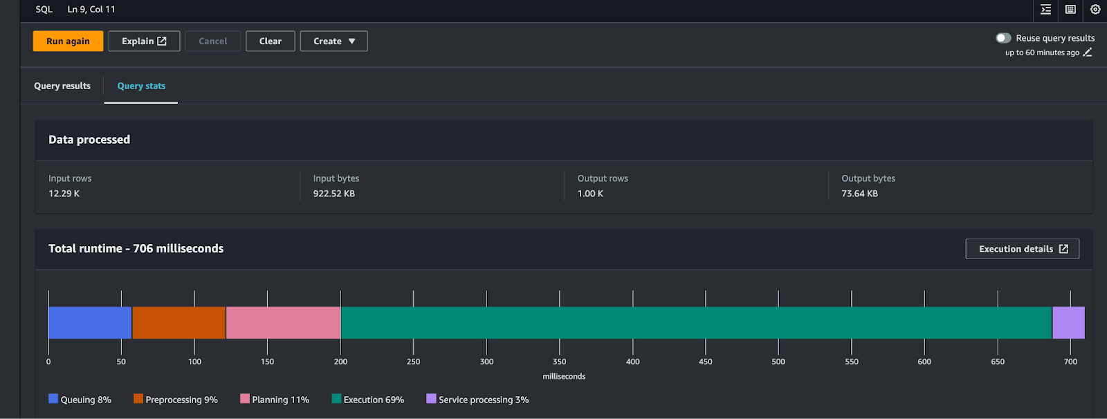
Limiting records (using the `LIMIT` keyword) does not preclude larger scans against the underlying objects in S3. To limit the amount of data returned, you use WHERE clauses to specify conditions – such as a time range, equality or negation, or a partition. Going forward, to monitor the performance of the queries, refer to the Query stats column within the Amazon Athena query editor results pane, as shown below (FIG. 1).
Building on the theme of specificity, to retrieve 1000 rows of hostname, username, and SHA256 hashes from endpoints with suspected malicious binaries, you can execute the following statement.
SELECT

    computername,

    ipv4_address,

    sha256_hash

FROM

    "pyspark_demo_db"."synthetic_edr_demo_raw"

WHERE

    severity_level = 'Malicious'

LIMIT 1000
My average runtime for this query was around 600ms, however, depending on how much data you generated, this can vary. You may have results where there is not any entry for the SHA256 hash. Additionally, using the LIMIT clause does not enforce or promise consistent ordering across different results.
Searching for IOCs
Investigations on EDR telemetry may occur when a new set of Indicators of Compromise (IOCs) is provided by your cyber threat intelligence (CTI) team. For instance, the SHA256 hash of 66fb3bfdb601414cd35623d3dab811215f8dfa08c4189df588872fb543568684 (W32/Fareit.A or Dino.zip) may have been recently surfaced by your CTI team. You could quickly search for this with the following statement.
SELECT

    computername,

    ipv4_address,

    sha256_hash

FROM

    "pyspark_demo_db"."synthetic_edr_demo_raw"

WHERE

    sha256_hash = '66fb3bfdb601414cd35623d3dab811215f8dfa08c4189df588872fb543568684'
In my result set, I received 268270 rows of data back, and my average run time was 2.65 seconds across 10 runs. Hopefully, in a real scenario you will not have gotten as much data back for a malicious indicator. Also, in a real scenario, you will likely have several indicators to search across, which is easily done in a limited set using the OR boolean operator after your initial WHERE keyword.
SELECT

    computername,

    ipv4_address,

    sha256_hash

FROM

    "pyspark_demo_db"."synthetic_edr_demo_raw"

WHERE

    sha256_hash = '66fb3bfdb601414cd35623d3dab811215f8dfa08c4189df588872fb543568684'

OR

    sha256_hash = '8bbd7978caf86b0f17690586225e296123d6664916e40a4b02a65cc605e4692b'

OR

    sha256_hash = 'c1aed0999337544d19ea857dc40743ec8b484c2d8ec6997207e5672539110b22'
On average, the runtime for this query for my dataset was 4 seconds and yielded 806773 results. Again, hopefully this wouldn’t happen in a real world scenario or you would have much bigger issues than query performance tuning! The syntax is incredibly verbose. Another way to perform this search is to use the IN keyword, which compares the field within your clause against values in a tuple as shown below.
SELECT

    computername,

    ipv4_address,

    sha256_hash

FROM

    "pyspark_demo_db"."synthetic_edr_demo_raw"

WHERE

    sha256_hash IN (

        '66fb3bfdb601414cd35623d3dab811215f8dfa08c4189df588872fb543568684',

        '8bbd7978caf86b0f17690586225e296123d6664916e40a4b02a65cc605e4692b',

        'c1aed0999337544d19ea857dc40743ec8b484c2d8ec6997207e5672539110b22'

    )
Using the IN keyword can greatly reduce the verbosity of a SQL statement and also improve its readability. However, it does not necessarily speed up the overall performance of the query given how much time is spent in query execution. Additionally, you can only compare data types in this way, such as specifying a tuple of strings against a field that is typed as a string.
Querying by Time
To further improve the performance of your queries, you should add a time box where you search. For this synthetic data, the timestamp format for first_seen_at was intentionally set to use Unix time for the purpose of demonstrating another concept in SQL: the SQL Function. SQL functions are built-in operations that support limited data type manipulation, data transformations, and other tasks without needing to use an external tool to further process your query results.
The from_unixtime() operator converts Unix time (Epoch seconds) into a timestamp data type. Without this conversion, the data is typed as a BIGINT within the Glue Data Catalog and timestamp comparators and operations are not compatible with that. While you can perform logical operations such as greater than or equal to a Unix timestamp, the lack of an (easily) human-readable timestamp can negatively affect comprehension, especially if these SQL statements are part of incident response playbooks.
The following statement adds the first_seen_at field to your results and uses the from_unixtime() operator on it; the AS keyword allows you to alias field names to dynamically change casing or terminology. Notice that the string which defines the date range you want to search from (in this case, 1 JANUARY 2024) is prepended with TIMESTAMP so it is not evaluated as a string.
SELECT

    from_unixtime(first_seen_at) AS first_seen_at,

    computername,

    ipv4_address,

    sha256_hash

FROM

    "pyspark_demo_db"."synthetic_edr_demo_raw"

WHERE

    sha256_hash IN (

        '66fb3bfdb601414cd35623d3dab811215f8dfa08c4189df588872fb543568684',

        '8bbd7978caf86b0f17690586225e296123d6664916e40a4b02a65cc605e4692b',

        'c1aed0999337544d19ea857dc40743ec8b484c2d8ec6997207e5672539110b22'

    )

AND

    from_unixtime(first_seen_at) >= TIMESTAMP '2024-01-01 12:00:00'
Depending on the size and distribution of your own dataset, you may not have noticed an improvement in query performance. In my case, this query took longer than not specifying time at all, on average 5.1 seconds. This is due to the additional compute cost and time within query execution to convert from Epoch seconds into a SQL timestamp.
This is also why partitioning your data is important, as the Glue Data Catalog is consistent with Apache Hive. The way to accomplish this is creating logical partitions in your storage layer (in this case, S3 folders) which group your data files in the same time range together. This S3 location is annotated within the partition data stored in the Glue Data Catalog which is passed along during the query planning stage. Partitioning greatly reduces the execution time as well – even with converting the time format – as Glue provides Athena-specific locations where files are found, instead of Athena scanning everything.
Before moving on, we can benchmark some other behaviors to compare after we partition this table. Let’s say you wanted to hunt for IOCs in reverse, instead of starting from a list of known-malicious IOCs, you can harvest every single unique IOC that your EDR flagged as suspicious or the endpoint team entered in a previous exception to. From there you can provide the result set to your CTI team, look up against a Threat Intelligence Platform (TIP), or otherwise.
Query for Uniqueness
To enforce uniqueness in SQL, you add the DISTINCT keyword to your DQL. This will return only unique entries of fields you specify. For searching a single field, this guarantees at-most-one results per unique entry. However, if you execute SELECT DISTINCT * when run against a large time-series table, you may still receive every single entry. Use due care when executing any DQL without narrowing your fields.
SELECT DISTINCT

    sha256_hash

FROM

    "pyspark_demo_db"."synthetic_edr_demo_raw"

WHERE

    severity_level IN ('Exception', 'Suspicious')
On average, this took 1.1 seconds within my dataset and returned 53 results, however there is some junk data within the synthetic data. For instance, the value “sha256” is included and the DISTINCT keyword returns all unique values even if they are empty (NULL).
How to Remove NULL Values
To remove NULL values you must use the IS NOT keyword, and to remove certain strings you use the not-equals operator (!=). If you had several values you did not want to include, you could alternatively use NOT IN and pass a tuple of the values of the same data type you do not want in your result set. In terms of matching equality or negation of it, values must be of the same types (e.g., string, integer, double, etc.) and strings are evaluated with case sensitivity by default, unless you use regular expressions.
SELECT DISTINCT

    sha256_hash

FROM

    "pyspark_demo_db"."synthetic_edr_demo_raw"

WHERE

    severity_level IN ('Exception', 'Suspicious')

AND

    sha256_hash != 'sha256'

AND

    sha256_hash IS NOT NULL
For my dataset the time average is around the same 1.1 seconds mark.
Counting in SQL
For the final scenario, you will audit the devices and a majority of the details going back six months that had a malicious or suspicious event. You will need to provide a count of the amount of times the device was implicated as well.
To do this in SQL, you use the COUNT() function which returns the number of rows (sum) that matches a specific condition. The condition is established by passing a wildcard or specific field name and takes into account any predicates or other conditions that you define. To count the unique instances of something, you can add the DISTINCT keyword inside of the COUNT() function to reference a wildcard or field name, as shown below.
SELECT COUNT(DISTINCT device_id) AS total_devices

FROM "pyspark_demo_db"."synthetic_edr_demo_raw"
In the above example take note that DISTINCT must be passed in front of your field name within the COUNT() function. The AS keyword is used to provide an alias for the results. Given that COUNT() is a function, it can be used within your DQL alongside other regular field names.
To add further complexity to the matter, anytime you reference more than one field name to use alongside a COUNT() function, you must also use the GROUP BY keyword. As COUNT() is an aggregation function, you use it with GROUP BY to group the same values into summary rows that help answer questions such as “customers in each country” or “amount of EDR findings by device”. You can also use GROUP BY on its own, but typically you’ll use it with aggregations.
Finally, to organize your results use the ORDER BY keyword to sort them ascending or descending. For integers, this is done numerically (obviously), but for strings they will be sorted alphabetically. You can reference different directions and different field names with ORDER BY. The ordering is applied in the order (no pun intended) they are specified.
Use the following statement to retrieve the computername (hostname), device ID, and total count of devices from 10 OCT 2023 that have reported “Malicious” or “Suspicious” findings.
SELECT

    computername,

    device_id,

    COUNT(device_id) AS total_times_seen

FROM

    "pyspark_demo_db"."synthetic_edr_demo_raw"

WHERE

    from_unixtime(first_seen_at) >= TIMESTAMP '2023-10-01 12:00:00'

AND

    severity_level IN ('Malicious', 'Suspicious')

GROUP BY

    device_id,

    computername

ORDER BY

    total_times_seen desc
Using GROUP BY and ORDER BY just requires referencing field names with the added benefit of ORDER BY being able to recognize aliases, as these aggregation tasks are applied towards the end of a transaction against the table. The performance of this query varied for me, but my data set finished with an average of 2.5 seconds, returned 24999 records, with the “leader” being hit 701 times. (ouch!)
In this section, you learned about SQL sublanguages and keywords and also put several keywords into practical usage. Additionally, you learned how to benchmark different queries and gained a foundational understanding of the influences on query planning and query execution. In the next section you will use EMR Serverless, Jupyter notebooks, and Apache PySpark to dynamically partition this data and create a new table.
Auto-Partition Data with PySpark
In this section, you will use EMR Serverless, Jupyter notebooks, and Apache PySpark to learn to dynamically convert data types, apply partitioning, and interpolate schema from the PySpark DataFrames to create Glue tables dynamically. From this new table you will repeat some of the SQL queries to check how much of a query performance improvement using partitions have on the queries.
IMPORTANT NOTE: Ensure you have accomplished all tasks within the Getting started with Amazon EMR Serverless section of the Amazon EMR Serverless User Guide to use an EMR Serverless application (with release version emr-6.15.0 and above) and EMR Studio.
A Jupyter notebook is an interactive environment that allows you to execute Python code, create markdown sections to add notes and observations, and you can also execute “magics” or shell scripts from the environment as well. Notebooks allow you to break Python code in several “blocks” which can be run independently of each other and also allow you to share context – such as libraries, constants, variables, and more – with other blocks of code in the notebook. Finally, notebooks can also retain the outputs of blocks to use as templates or as evidence of a successful run.
Notebooks are typically used by data engineers and data scientists for creating prototypes and exploratory data analyses but are also a popular choice for detection engineers and SecDataOps practitioners to define runbooks and playbooks as code. You can use notebooks to provide clear instructions for incident response, threat hunting, internal investigations, or red teaming exercises for junior members of a team or to guarantee a repeatable process. The modularity of code blocks allows you to import additional libraries or change variables on the fly if a situation arises.
The drawbacks to notebooks is the rigidity of the kernels, you can only import libraries that are prepackaged and the “magics” may not be available to allow you to install them as required. Additionally, they can become unmanageable very quickly as the blocks expand within them, whereas Python programs can be built out horizontally with your own classes and libraries to expand usage and readability. Ultimately, their usage is up to the individual SecDataOps team, but learning their usage is very valuable.
NOTE: If you already have experience with Jupyter notebooks and can make the necessary changes to the script, you can download the template from here. If you wish to follow along, you can still download the template but we will walk you through the various sections of the notebook and provide the code snippets in the body of the blog as well.
How to Launch a Notebook
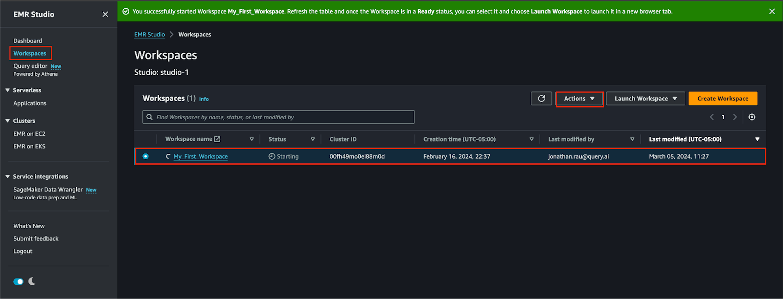
Step 1. Navigate to the Amazon EMR console, select Workspaces, and start your Workspace as shown below (FIG. 2). When the Status changes to Ready, you launch a new browser window to interact with EMR Studio.
Step 2. The EMR Studio Workspace is a hosted JupyterLab environment that allows you run various Notebooks, create a shell, author other types of files and scripts, or run SQL queries. Select the PySpark option from the Notebook header as shown below (FIG. 3).
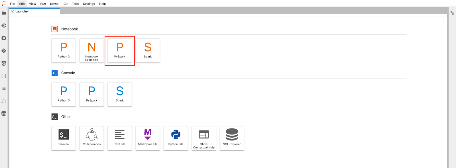
Once your notebook has been created, it will establish a kernel that can take a few minutes to instantiate.
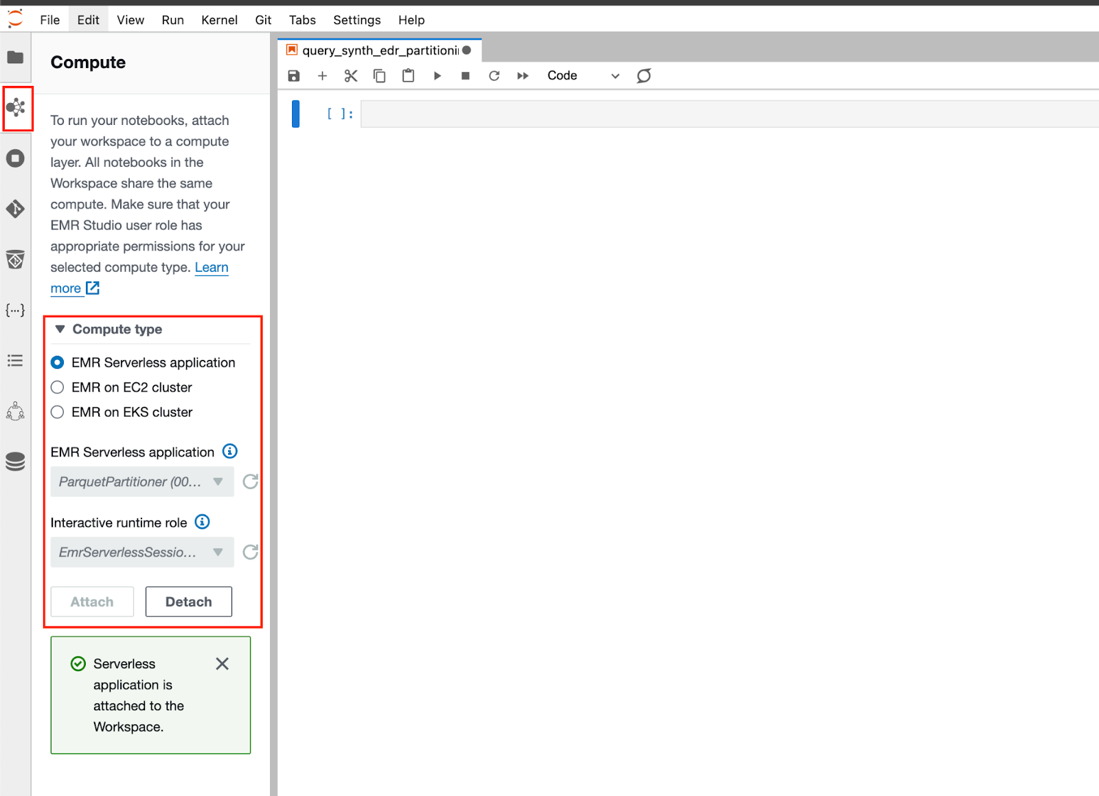
Step 3. On the left-hand navigation pane, open the Compute section denoted by the Amazon EMR service icon. Select EMR Serverless application for your Compute type and select your EMR Serverless application and Interact runtime role that you set up in the prerequisites, as shown below (FIG. 4). Your runtime role should have access to AWS Glue APIs as well as the Amazon S3 bucket (and objects) you worked with in the previous sections.
To add a new block into the notebook, select the plus (“+”) icon from the interface at the top of the screen. By default these are code blocks, we will not be adding any markdown at all. To execute the code within the block, select the “play button”. Results of the block are printed below the block, as shown below (FIG. 5).
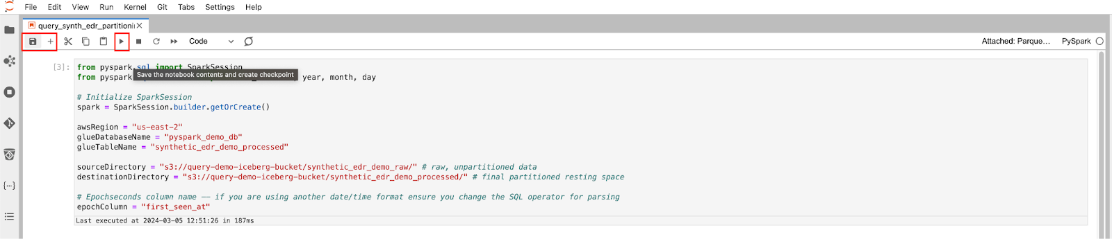
Ensure you periodically save as you go in case you lose internet connection. To start, paste the following Python code into the first block.
Block 1
from pyspark.sql import SparkSession

from pyspark.sql.functions import from_unixtime, year, month, day, col, to_timestamp

# Initialize SparkSession

spark = SparkSession.builder.getOrCreate()

awsRegion = "us-east-2"

glueDatabaseName = "pyspark_demo_db"

glueTableName = "synthetic_edr_demo_processed"

sourceDirectory = "ss3://query-demo-iceberg-bucket/synthetic_edr_demo_raw/" # raw, unpartitioned data

destinationDirectory = "s3://query-demo-iceberg-bucket/synthetic_edr_demo_processed/" # final partitioned resting space

# Epochseconds column name -- if you are using another date/time format ensure you change the SQL operator for parsing

epochColumn = "first_seen_at"
This first code block will import the required dependencies, instantiate a Spark session, and set several variables that will be reused throughout the notebook. Ensure you change the values as required to match your own AWS region, database, table, and bucket names. The value of destinationDirectory will be automatically created for you. While it is possible to overwrite and partition-in-place with PySpark – we will not be doing that in this blog entry.
Lastly, ensure that the column that contains Unix time is correct, this is the default value unless you greatly modified the synthetic data script. Notice that we imported the from_unixtime method from pyspark.sql.functions which is a 1:1 representation of the built-in SQL from_unixtime() function. This notebook could theoretically be converted to use for other tables with Unix time or changed to account for different types of time conversions. Paste the following Python code into a new block and execute it.
Block 2
# Load DF, convert Epochseconds to timestamp

df = spark.read.format("parquet").option("compression", "zstd").load(sourceDirectory)

df = df.withColumn(epochColumn, from_unixtime(epochColumn))

# Extract year, month, and day from epoch seconds column for partitioning

df = df.withColumn("Year", year(epochColumn))

df = df.withColumn("Month", month(epochColumn))

df = df.withColumn("Day", day(epochColumn))
This code block creates a PySpark DataFrame (variable of df) by using the Spark session to read the Zstandard-compressed Parquet objects from the source directory in S3 you specified. There is self-referential code that continues to sequentially update the DataFrame, which is why you see df = df.some_method various times. The second line converts the Unix time column into a SQL timestamp data type.
Following that, the columns for Year, Month and Day are created using that newly-converted timestamp column with the other functions that were imported in the first block. This is how Spark will know which partitions to create and how to reference them when you create the Glue table and add the partitions into it. Remember, Glue tables are essentially Hive tables and require explicit columns that refer to partitions.
Glue Data Catalog requires storage location references for each partition combination as well, for instance, for the partition of /year=2024/month=01/day=02 the full S3 URI denoting that path needs to be added. In this way, the Glue Data Catalog can fully instruct Athena where to download and read S3 objects corresponding to that partition. Paste the following Python code into a new block and execute it to progress.
Block 3
from pyspark.sql.types import TimestampType

# ensure that converted time column is cast as a timestamp correctly

df = df.withColumn(epochColumn, to_timestamp(epochColumn).cast(TimestampType()))

# write out to destination in append mode

df.write.partitionBy("Year", "Month", "Day").format("parquet").option("compression", "zstd").mode("append").save(destinationDirectory)

# read the unique partitions

df = spark.read.format("parquet").load(destinationDirectory)

partitions = df.select("Year", "Month", "Day").distinct().collect()

# read the schema

schema = df.schema

print(schema)
First, we ensure that the column we converted from Unix time to a SQL timestamp is properly typed as a timestamp. Then you write the data with your specified partitions (Year, Month, Day) to your S3 destination variable location. We also explicitly define that the data should remain in Zstandard-compressed Parquet files with the “append” mode of operation which would append data to existing data. The other mode commonly used is “overwrite” which would replace all of the files.
The last parts of the script read back the newly partitioned data to retrieve the unique values from the Year, Month and Day partitions along with the schema for the table. This will be passed over to the Boto3 client for AWS Glue to create a new table for the partitioned data that you can query. Paste the following Python code into another block and run it to continue to move on.
Block 4
# setup deps for creating Glue Table

import boto3

from pyspark.sql.types import *

glue = boto3.client("glue", region_name=awsRegion)

# convert Spark DF types -> Athena engine v3 (Trino-ish?) types

def sparkDataTypeToAthenaDataType(sparkDataType):

    mapping = {

        IntegerType: "int",

        LongType: "bigint",

        DoubleType: "double",

        FloatType: "float",

        StringType: "string",

        BooleanType: "boolean",

        DateType: "date",

        TimestampType: "timestamp",

    }

    return mapping.get(type(sparkDataType), "string")  # Default to string type if unknown
This code imports Boto3 and sets up the client for AWS Glue and defines a function that is used to map notable Spark DataFrame data types into SQL data types supported by Amazon Athena. For any data type not explicitly defined, it will default to a string. Ensuring the proper typing of data leads to increased memory efficiency and thus query performance. This function will be called later in the note. Proceed to add and execute the following code snippet to another code block.
Block 5
def getGlueTableColumns(schema, partitionKeys):

    columns = []

    for field in schema.fields:

        if field.name not in partitionKeys:  # Skip partition keys

            athenaDataType = sparkDataTypeToAthenaDataType(field.dataType)

            columns.append({"Name": field.name, "Type": athenaDataType})

    return columns

def createGlueTable(glueDatabaseName, glueTableName, columns, partitionKeys, destinationDirectory):

    glue.create_table(

        DatabaseName=glueDatabaseName,

        TableInput={

            "Name": glueTableName,

            "StorageDescriptor": {

                "Columns": columns,

                "Location": destinationDirectory,

                "InputFormat": "org.apache.hadoop.hive.ql.io.parquet.MapredParquetInputFormat",

                "OutputFormat": "org.apache.hadoop.hive.ql.io.parquet.MapredParquetOutputFormat",

                "SerdeInfo": {

                    "SerializationLibrary": "org.apache.hadoop.hive.ql.io.parquet.serde.ParquetHiveSerDe",

                },

            },

            "PartitionKeys": [{"Name": key, "Type": "string"} for key in partitionKeys],

            "TableType": "EXTERNAL_TABLE"

        }

    )

# get the columns, sans partitions

partitionKeys = ["Year", "Month", "Day"]

columns = getGlueTableColumns(schema, partitionKeys)
This code block defines two more functions. The first (getGlueTableColumns()) collects all of the column names from the DataFrame schema, properly sets their data type, and ignores the partition column names. The second function (createGlueTable()) is called later and will take in several variables you defined, columns, and partition names to create a new Glue table based on the newly partitioned data. Paste the next snippet into a new block and execute it to continue.
Block 6
try:

    c = createGlueTable(glueDatabaseName, glueTableName, columns, partitionKeys, destinationDirectory)

    print("table create successfully")

    print(c)

except Exception as e:

    raise e
This snippet will call the function that creates the new Glue table. If you lack the proper permissions, this block will completely fail. Now that you have a new table, you have to add the actual partition data into it. As noted earlier, Glue Data Catalog requires the S3 path (location) for each partition. Right now there are only the names of the partitions noted within the table. To add that partitioning information in bulk, proceed to paste the penultimate code block and execute it.
Block 7
def addPartitionsToTable(glueDatabaseName, glueTableName, partitions, destinationDirectory):

    partitionInputs = []

    for partition in partitions:

        year, month, day = partition["Year"], partition["Month"], partition["Day"]

        # Construct the s3 uri for this specific partition

        partitionLocation = f"{destinationDirectory}/Year={year}/Month={month}/Day={day}"

        partitionInput = {

            "Values": [str(year), str(month), str(day)],

            "StorageDescriptor": {

                "Columns": [],  # This can be empty as columns are defined at the table level

                "Location": partitionLocation,

                "InputFormat": "org.apache.hadoop.hive.ql.io.parquet.MapredParquetInputFormat",

                "OutputFormat": "org.apache.hadoop.hive.ql.io.parquet.MapredParquetOutputFormat",

                "SerdeInfo": {

                    "SerializationLibrary": "org.apache.hadoop.hive.ql.io.parquet.serde.ParquetHiveSerDe"

                }

            }

        }

        partitionInputs.append(partitionInput)

    # Use the AWS Glue client to batch create partitions

    try:

        glue.batch_create_partition(

            DatabaseName=glueDatabaseName,

            TableName=glueTableName,

            PartitionInputList=partitionInputs

        )

    except Exception as e:

        raise e

def createUniqueChunks(data, maxPartitionCount=95):

    unique_data = list(set(data))  # Remove duplicates to ensure uniqueness

    chunks = [unique_data[i:i + maxPartitionCount] for i in range(0, len(unique_data), maxPartitionCount)]

    return chunks

def partitionAndProcess(data):

    if len(data) > 95:

        chunks = createUniqueChunks(data)

        for chunk in chunks:

            addPartitionsToTable(glueDatabaseName, glueTableName, chunk, destinationDirectory)

    else:

        process_chunk(data)

# Using the partitions collected from your DataFrame - split them if there are more than 95 and bulk add the data to the table

partitionChunk = partitionAndProcess(partitions)
This snippet first establishes the function (addPartitionsToTable()) that is used to bulk add partitions and define the S3 paths that correspond to them. You can only write in batches of 100 into AWS Glue, so the following functions will check the length of all partitions created by PySpark and create chunks of 95 partitions to add into your table at a time. Depending on the distribution of the data you generated, you could have several 100 partitions. I have 295 in my own dataset.
Block 8
Finally, to stop the Spark session and proceed to the next section, run the following command in your notebook.
spark.stop()In this section, you learned how to navigate EMR Studio to create a Jupyter notebook with a PySpark kernel and how to navigate the elements within it. Additionally, you learned how to mount a session and provide IAM Role-derived permissions to your runtime environment. You also learned how to define PySpark DataFrames, perform large scale bulk operations on data types, and dynamically created partitions. Finally, you learned how to use the outputs of a DataFrame for follow-on operations using AWS’ native Software Development Kit (SDK).
In the next section, you will run through benchmarking some of the SQL statements you ran in the previous sections against this newly partitioned table before we close out this blog entry.
Querying Partitioned Tables
In this section, you will perform a subset of the queries against the partitioned synthetic EDR telemetry data table to learn how to use them in Athena. At the end of this section you should be able to determine if partitioning improves performance for you versus not.
After shutting down the EMR Serverless resources (and optionally deleting them), proceed back to the query editor in the Amazon Athena console. One of the first complex SQL statements you issued was looking for known-malicious SHA256 hashes from 1 JAN 2024 onwards. To modify that statement to use partitions, you specified them as part of the WHERE clause. Additionally, you also transformed the Unix time column into a proper SQL timestamp, so a conversion is not required. Execute the following statement 5 to 10 times to see if it is consistently faster than before.
SELECT

    first_seen_at,

    computername,

    ipv4_address,

    sha256_hash

FROM

    "pyspark_demo_db"."synthetic_edr_demo_partitioned"

WHERE

    year = '2024'

AND

    sha256_hash IN (

        '66fb3bfdb601414cd35623d3dab811215f8dfa08c4189df588872fb543568684',

        '8bbd7978caf86b0f17690586225e296123d6664916e40a4b02a65cc605e4692b',

        'c1aed0999337544d19ea857dc40743ec8b484c2d8ec6997207e5672539110b22'

    )

AND

    first_seen_at >= TIMESTAMP '2024-01-01 12:00:00'
For my dataset, the previous raw table had an average time of 5.1 seconds and brought back 189,657 records. The partitioned table averaged closer to 2.4 seconds and brought back the same amount (it should have!). While this varies greatly based on the amount of data and partitions, that is a little under twice as fast to return results. That is not to suggest the performance is linear, and there are a lot of factors that can influence the outcome.
Another observation is that querying the partitioned tables has a slightly higher time spent in planning than execution. This is because you do not call any SQL function to perform a data type conversion, and the WHERE year = ‘2024’ clause helps Athena make use of the S3 location information in the Glue data catalog. It can ignore any 2022 or 2023 year entries completely, which lends itself to faster query performance and lowered costs.
For a final example, let’s modify the aggregation query where we attempted to get a total count of each device implicated in a “Malicious” or “Suspicious” finding from 1 OCT 2023 and onward. We can put together several partitions in our query to further specify which months to use in addition to which years. Modify your query as required – this blog post was written in March 2024.
SELECT

    computername,

    device_id,

    COUNT(device_id) AS total_times_seen

FROM

    "pyspark_demo_db"."synthetic_edr_demo_partitioned"

WHERE

    year = '2023' OR year = '2024'

AND

    month IN ('10','11','12','01','02','03')

AND

    first_seen_at >= TIMESTAMP '2023-10-01 12:00:00'

AND

    severity_level IN ('Malicious', 'Suspicious')

GROUP BY

    device_id,

    computername

ORDER BY

    total_times_seen desc
On average, this query was about the same as it was against the unpartitioned table, about 2.5 seconds to complete. While we made up time without having to convert Unix time into a timestamp to begin the comparison, there is another force working against us, as this is an aggregation function that works across several months. Remember that in data lakes the “small file problem” can add processing time to queries as several objects must be downloaded and read by Athena. While our original table was not partitioned, we only had a few files to contend with, when using PySpark to apply partitions it wrote the files into smaller, separate files increasing the total amount.
There is some work you can do, such as lessening the amount of partitions – for example, getting rid of the “Day” partition – or you can create automation for compaction tasks that will combine files in batches of 240MB per file. Ultimately, your data access patterns and detection use cases should influence the amount of partitions you create and how to manage these smaller data files. For that reason, you may find that not using partitions at all is perfectly fine where other data may require the usage of partitions. You may also find that partitioning by year or month on their own is fine, but other tables may require hourly partitions, especially if you want to perform complex detections as soon as possible after data is written.
What Should You Do?
Carry forth this work to benchmark your performance and use the PySpark script to create new tables with partitions for it. In my experience, when querying “fact tables” such as assets or inventory, it almost never makes sense to partition it unless you keep records day over day. For high volume data such as network flows, DNS, web application firewalls, or Windows Events it may make sense to perform hourly partitioning especially if you want to run a query every single hour to hunt for tradecraft or IOCs. Of course, the best move you can make is to use Apache Iceberg, which helps you automate partitioning and compaction of data a lot easier than using PySpark or otherwise.
Stay Dangerous.